The Effect of Monetary Policy Assumptions on Fiscal and Macroeconomic Analysis
Over the last several decades, budgetary analysis has moved beyond first order fiscal effects and increasingly incorporated macro- and microeconomic feedback. This shift towards dynamic, general equilibrium modeling has made fiscal analysis more complex, but also more economically-complete and—hopefully—more informative to policymakers and the general public.
The added complexity of dynamic analysis also means new assumptions and sources of uncertainty. One of the cornerstone assumptions in macroeconomic modeling is the reaction of the central bank to a policy shock. In the US context, this is key since the Federal Reserve is politically independent, and so may attempt to mitigate the economic effects of a fiscal intervention. The Fed’s possible intervention, or not, has major implications for the trade-offs of an economic policy. That means in turn, that the Federal Reserve’s independence also has major implications for how fiscal policy impacts the economy.
This question is not purely theoretical. The Federal Reserve has not always been politically independent throughout its history. In the early 1970s, President Nixon pressured then-Fed Chair Arthur Burns to keep monetary policy easy as Nixon was running for reelection. Burns acquiesced even though inflationary pressures that had arisen in the late-1960s were persisting. When the oil crisis hit in 1973, these ongoing pressures added to the new inflationary pressures driven by the energy supply shock. The result was the stagflation of the 1970s.
Here we review how the Federal Reserve often responds to fiscal policy and what the implications of a non-independent Federal Reserve would be.
A simple example: a tax cut under full employment
Take for example a simple illustrative tax cut enacted in 2024 that permanently reduces federal revenue by 1% of GDP a year. Since the US economy is currently at full employment, a reasonable economic conclusion is that this policy would bolster demand such that there are more claims to the already-fully-utilized real resources of the economy. This adds to inflationary pressure in the short-run. But whether the actual outcome of the policy would be higher realized inflation depends on the Fed’s reaction. The Fed could do nothing in response to the tax cut, in which case the trade-off would indeed primarily be higher realized inflation. More likely, the Fed would raise interest rates or otherwise tighten monetary policy in response to the inflationary pressure of the tax cut. This would offset that pressure in line with the Fed’s price stability mandate. In that latter scenario, the trade-off of the tax cut in actuality would not entirely be higher realized inflation, but instead involve higher interest rates, an economically-distinct outcome in important ways.
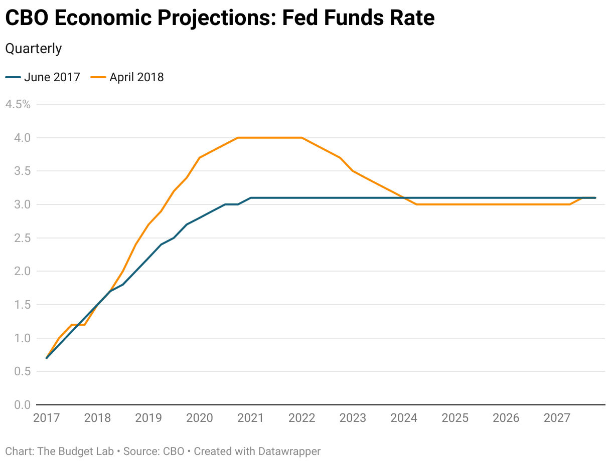
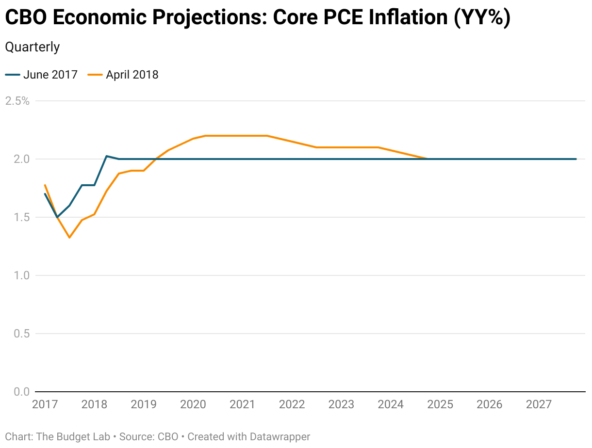
In fact, there is a recent real-world example of almost exactly this scenario: the Tax Cuts and Jobs Act (TCJA). The TCJA was a large tax cut passed in December 2017, when the economy was already close to full employment (the unemployment rate that month was 4.1%). From the standpoint of first principles, then, a macroeconomist would have assumed that the law would have added to inflationary pressure in the near term. But when the Congressional Budget Office (CBO) updated their economic projection after the law’s enactment, their inflation outlook only rose slightly in the short-run (Figure 1 below, right panel). Instead, CBO assumed the Federal Reserve would react to the TCJA’s inflationary pressure and temporarily raise interest rates to neutralize the added inflation risk (Figure 1, left panel). If instead CBO had assumed no monetary policy reaction to the TCJA, they likely would have shown more trade-off with inflation.
Figure 1.
Indirect Taxes and the Price Level
As described above, aggregate demand is one channel through which tax policy affects inflationary pressures. Another channel involves so-called “indirect” taxes, a category which includes excise taxes, tariffs, retail sales taxes, and—in other countries—value added taxes (VATs). It is commonly understood that these kinds of taxes increase consumer prices, but it’s worth understanding exactly how this works and what role the Fed plays.
Most revenue in the United States is raised through what are known as direct taxes—taxes which are levied on the net income of households and firms, such as individual income taxes, employee-side payroll taxes, or corporate income taxes. Indirect taxes, on the other hand, are assessed on the production of goods and services. A key feature of indirect taxes is that they are applied at the firm level but do not allow a deduction for the cost of labor. This design creates a wedge between the wage employers are willing to pay and the wage that workers are willing to accept. In a TaxNotes piece on this topic, Alan Viard illustrates this dynamic using an example where a worker can produce 100 widgets sold for $100 each:
A VAT, however, reduces the short-run market clearing level of real wages because businesses are taxed on the value of their workers’ output without being allowed to deduct wages paid. A VAT imposed at a 10 percent (tax-inclusive) rate therefore reduces the real value of the worker’s labor to the employer by 10 percent, just as the 10 percent employer payroll tax did. If the Federal Reserve does not accommodate the VAT and the price of widgets remains at $100, the employer clears only $90 for each widget that is sold, with the other $10 paid in tax. Because the 100 widgets produced by the worker are now worth only $9,000 to the employer, the market-clearing wage falls to $9,000.
He contrasts this example, in which wages are non-deductible, with a business income tax:
Consider a 10 percent tax on the widget producer’s business income and assume that the Federal Reserve takes no action, leaving the price of widgets at $100. The business income tax reduces each widget’s net value to the employer from $100 to $90, just as the VAT and the retail sales tax did, because 10 percent of the widget sale proceeds are taxed away. Like the VAT and the sales tax, the business income tax therefore reduces the amount that employers are willing to pay out of pocket for each worker from $10,000 to $9,000. Nevertheless, the market-clearing wage remains unchanged at $10,000. Because the $10,000 wage payment can be deducted against the 10 percent business income tax to yield a $1,000 tax savings, the out-of-pocket cost of the wage payment is only $9,000.
This wedge between pre-tax and post-tax wages can resolve in one of two ways: the new tax burden is either “passed backwards” in the form of lower nominal wages, or “passed forward” to consumers in the form of higher prices. Because the Fed takes fiscal policy as given and is the "last mover” among factors which determine the price level, which of these two scenarios occurs is ultimately up to the Fed. In this sense, indirect taxes are not inflationary per se—rather, they create economic costs which the Fed, in fulfilling its mandate, may choose to resolve in the form of allowing a higher price level.1
If the Fed ignores an indirect tax increase by keeping total nominal spending on its current growth path, wages will fall. In this scenario, consumer prices stay fixed and the tax burden manifests as a loss of income. The alternative reaction is for the Fed to “accommodate” the tax hike by keeping nominal interest rates and balance sheet policy unchanged and allowing for a one-time increase in the price level. In this situation, nominal wages would be unchanged, but their real purchasing power would fall by the same amount as in the pass-backward case. In this sense, the pass-backward and pass-forward scenarios are identical from a microeconomic point of view.
At the level of macroeconomic decision-making, however, these scenarios have important differences which could impact how the Fed reacts. One consideration is cultural: workers simply do not favor nominal wage cuts, a phenomenon known as downward nominal wage rigidity. Another concern with the pass-backward scenario is that falling nominal incomes pose macroeconomic stability risks when debt contracts are widely denominated in nominal terms. For example, households take out mortgages under the expectation of positive nominal income growth and may be unable to make payments if wages fall. Lower nominal incomes might jumpstart a pernicious cycle of defaults, layoffs, and loss of output. Yet the pass-forward scenario is not without macroeconomic risks: large increases in the price level may cause an unanchoring of inflation expectations. In the case of a small tax increase, these factors may be too small to even notice in the context of normal monthly variation in the rate of inflation. But in the case of a large tax increase, such as the introduction of a VAT, these differences become meaningful. Interational evidence suggests that policymakers generally favor the pass-forward approach, as central banks in peer countries tend to “look through” price changes caused by VAT reforms.2
The implications of a “captured” central bank
The political independence of the Federal Reserve means that economists typically trust it will reliably react to shocks that affect its dual mandate. But the Fed’s political independence is not always expedient for political leaders. If for example a fiscal policy meant to boost demand is inflationary, an independent Fed will try to counteract it, mitigating its economic benefits and potentially raising the unemployment rate. Leaders may therefore be tempted to apply political pressure to the Fed as a way to curb its counterreaction. This may occur in many different ways, such as public threats to fire leadership or appointing loyalists to open Fed leadership positions.
A “captured” Fed would therefore be one less responsive to inflationary impulses, which allows inflationary pressure to build unchecked. To test the implications of capture, we ran a monetary policy rule that allows for a spectrum of political “capture”3 through a series of stochastic simulations in FRB/US, the Fed’s workhorse macroeconomic model.4 In these simulations, FRB/US picks random historical economic shocks to key variables occurring between 1970 and 2023 and applies them to its forward forecast. We ran 1,000 such simulations each assuming C = 0 (no political capture) and alternatively C = 0.85 (high political capture). C = 1 implies extreme perfect capture, in which the Fed only responds asymmetrically to low inflation and high unemployment.
Figure 2 illustrates the results. The x-axis shows cumulative 6-year inflation, while the y-axis denotes the probability of each outcome in our simulations.
A captured Fed skews economic outcomes towards more inflation over time. In our simulations, low inflation was just as likely under our two capture assumptions. But the median inflationary outcome was +0.6 percentage point higher after six years under high capture. And the outlier 95th percentile outcome was almost 2 percentage points higher under high capture (solid orange line).
Figure 2.
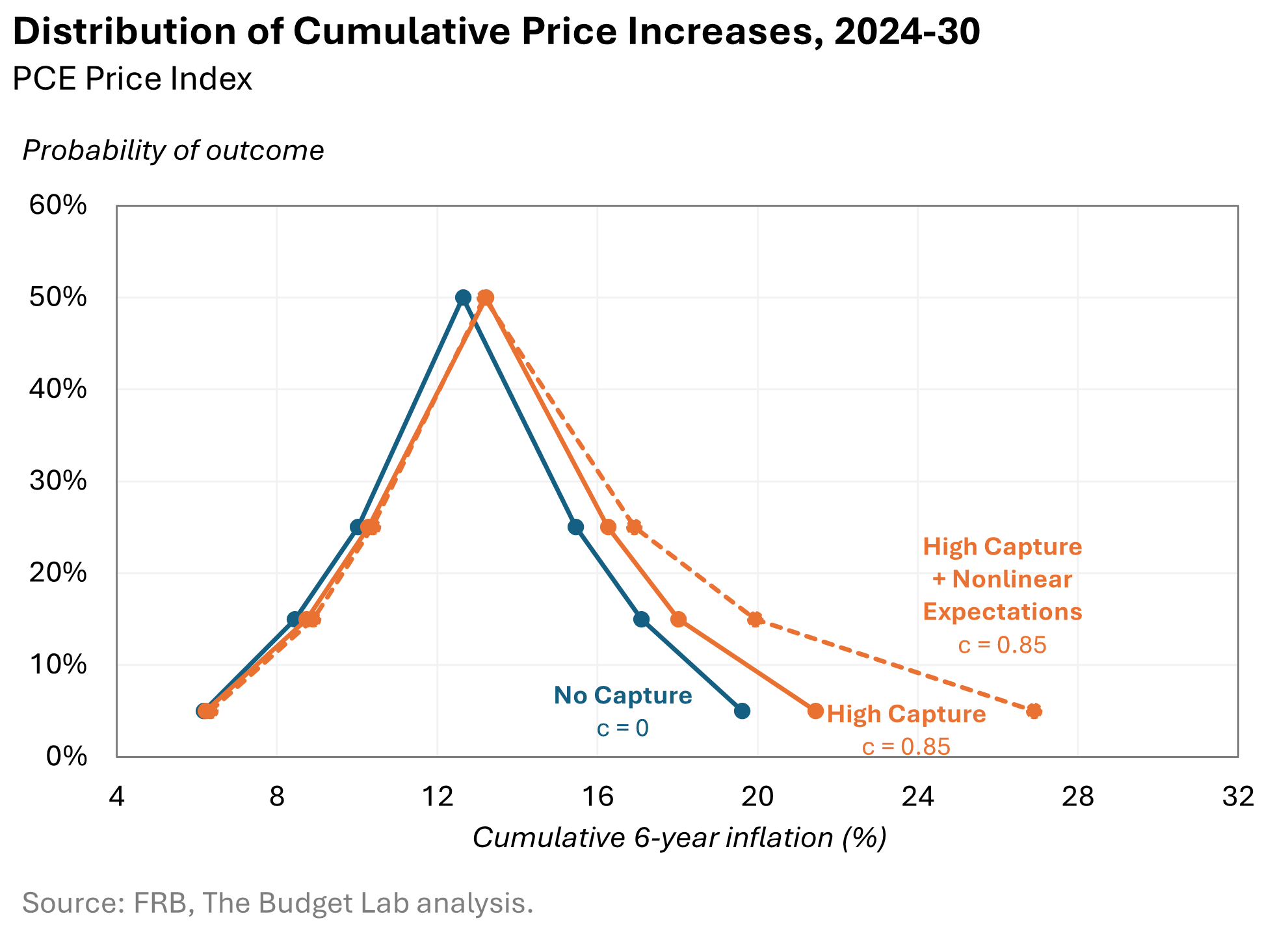
FRB/US also makes an important assumption: that even if inflation grows, the Federal Reserve retains credibility with consumers and markets. Put another way, inflation expectations remain tightly and linearly anchored to the Federal Reserve’s inflation target. But this may not reflect reality. If the Fed demonstrates it is unwilling to counter high inflation, inflation expectations may shift to a new regime that reflects a captured Fed. The dashed orange line in Figure 2 illustrates one way of simulating this possibility: so long as inflation stays below 3%, inflation expectation stay anchored to the Fed’s target. But above 3% inflation, expectations start becoming adaptive: they reflect actual lived inflation rather than Fed policy. These higher inflation expectations create space for even higher actual inflation. As Figure 2 shows, the potential for loss of Fed credibility makes the upside inflation risk considerably higher: an additional five percentage points in our simulations over six years.
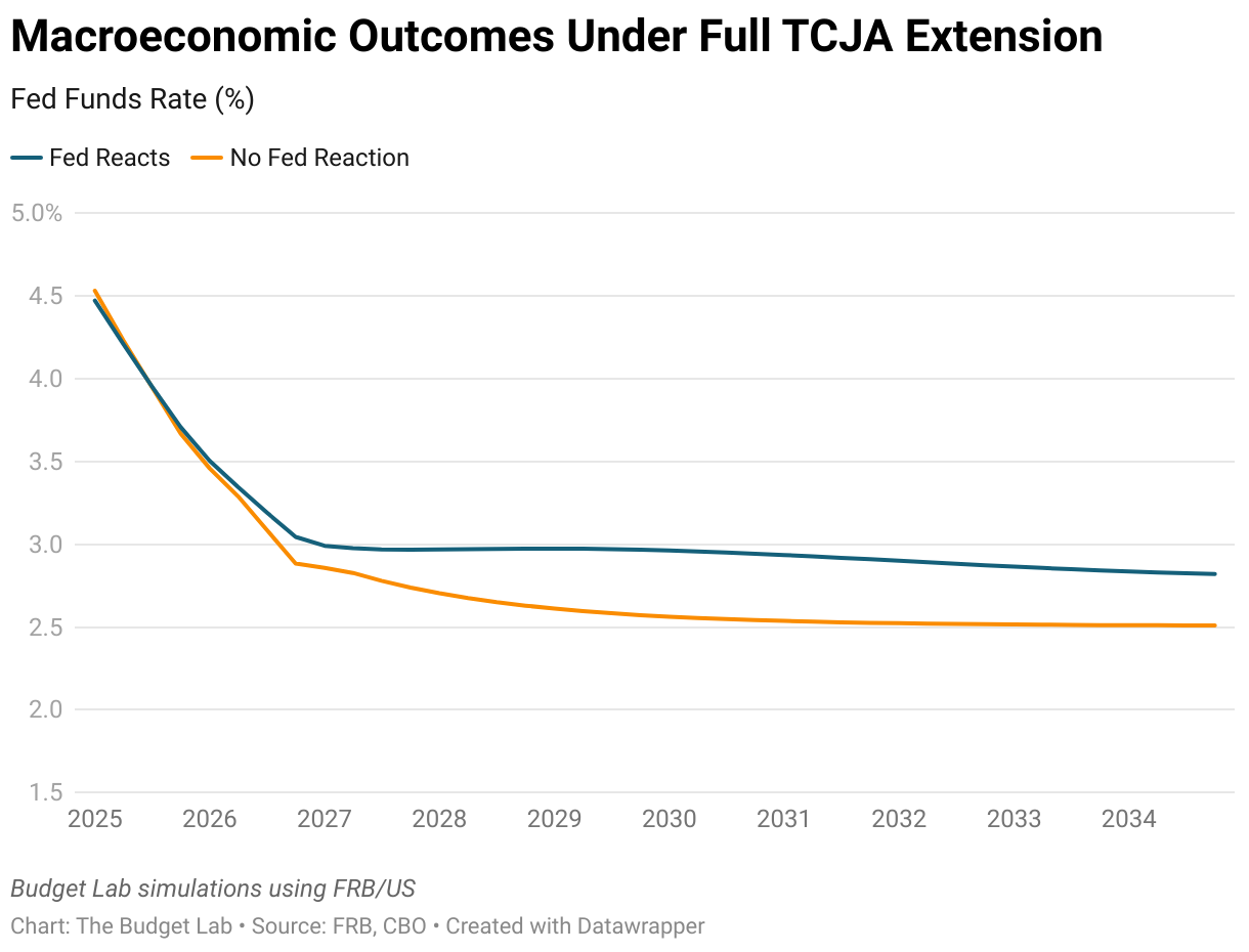
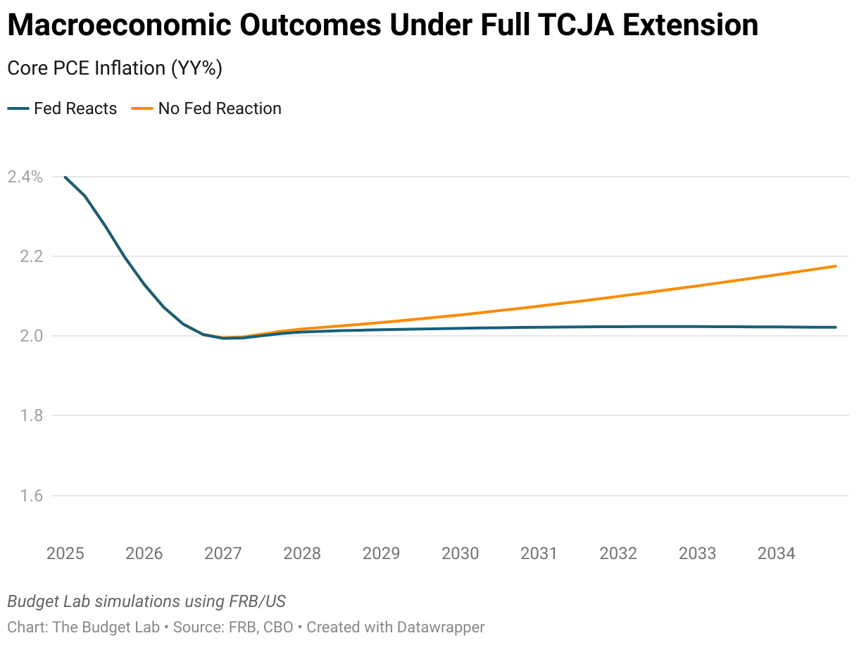
The importance of the Fed to economic outcomes is also evident when considering the debate around the upcoming extension of the individual provisions of the TCJA. Extending some or all of these provisions would represent fiscal impulse and could add to inflationary pressure (relative to current law) if the US is economy in 2026 is still at full capacity. The Budget Lab simulated full extension of the TCJA both with and without reaction from the Federal Reserve, using the Federal Reserve’s workhorse macroeconomic model FRB/US.5 The results in Figure 3 show the macroeconomic stakes around how reactive the Fed would be. If the Fed raised rates in reaction to the TCJA’s impulse (blue line, left panel), then it would effectively neutralize excess inflation (blue line, right panel). But if it did not react (orange line, left panel), interest rates would be lower but inflationary momentum would gradually build above the Fed’s 2% target (orange line, right panel). Bear in mind that both lines assume FRB/US’s standard linear, anchored inflation expectations; if expectations suddenly became unanchored, the inflation consequences would be more serious.
Figure 3.
What these exercises shows is that the loss of Federal Reserve independence is not an academic consideration. When the Fed is less responsive to nascent inflationary pressures, those pressures build over time. Price levels are likelier to be higher, making consumers worse off. Moreover, when inflation consistently runs above target without the Fed reacting, the Fed loses credibility, making future monetary policy even less effective.
Footnotes
- Targeted indirect taxes like excise taxes and tariffs my increase consumer prices for certain goods and services. These price increases, though, are relative price changes, not changes in the over price level, and so should not be thought of as constituting inflation.
- See Tait (1988) for a list of case studies.
- More specifically, we simulated a Fed reaction function of the following form:
Fed Funds Ratet = (1-C)*[rstart + 1.5*πt – 0.5*π· + ygapt] + (C)*[rstart + πta + ygapta]
Where
C is the amount of “capture,” measured between 0 and 1
πt is the year-on-year core PCE inflation rate
π· is the Fed’s inflation target (2%)
ygapt is the output gap
πta is the year-on-year core PCE inflation rate capped at 2%
ygapta is the output gap, capped at 0 (i.e. the Fed only reacts if the gap is negative/recessionary)
The function following (1-C) is a standard Taylor (1999) rule for the stance of the monetary policy. Therefore, when C = 0, the whole equation becomes a conventional reaction function. The piece following (C) is designed to be asymmetric: the Fed only reacts to low inflation, not high, and only to negative output gaps, not positive. - Expectations in FRB/US simulations are a linear function of either past actual (adaptive expectations) or future forecast (rational expectations) inflation. This linear characteristic of FRB/US expectations can often make inflation appear slow to respond to fiscal shocks in the model, even without a Federal Reserve response. By contrast, one risk with a captured Federal Reserve is a nonlinear deterioration in the Fed’s credibility and in inflation expectations: that expectations go from being strongly anchored around 2% to being hardly anchored at all in a short amount of time. That means the simulation results in this analysis may understate both the magnitude and the volatility of inflation outcomes under a captured Federal Reserve.
- The Budget Lab modifies FRB/US to conform to CBO’s fiscal baseline. See Budget Lab (2024) for more information.