The Impact of TCJA Reform on the Federal Budget
Key Takeaways
-
Fully extending the expiring provisions of the Tax Cuts and Jobs Act would increase primary deficits by more than 40 percent over the next decade, or about 0.7 percent of GDP.
-
The Partial Extension scenario has an average annual budget cost over the decade of 0.6 percentage point of GDP, with slightly smaller effects in the longer run.
-
The Clausing-Sarin reform cuts average annual primary deficits by nearly two-thirds. It raises 1.3 percentage points of GDP of new revenues on average over the decade, with more substantial savings in subsequent years.
Types of budget scores
We produce three types of budget estimate:
- A conventional revenue estimate, the kind produced by government scorekeepers at CBO and the Joint Committee on Taxation (JCT), measures both the mechanical (or “static”) change in revenues attributable to changes in tax law, as well as changes in revenues owing to tax avoidance responses. Crucially, these responses do not reflect substantive economic decisions which could have macro-level implications. Instead, behavioral responses in a conventional estimate are limited to a narrower set of tax optimization decisions: when to realize income, through what legal form to characterize business activity, in which sectors to invest, and so forth.1
- A microeconomic feedback estimate relaxes the assumptions of a conventional estimate by accounting for first-order changes in economic decisions, but not allowing for additional rounds of macroeconomic feedback. For example, an increase in payroll taxes might cause some workers to exit the labor force. This decline is a “first-order” economic effect and might be followed by second-order effects: employers might raise wages to attract new workers, the Federal Reserve might lower interest rates (which in turn might spur investment), and so on. In this case, a microeconomic feedback estimate would capture only the forgone tax liability associated with first-order employment changes, not any other potential changes. In other words, microeconomic feedback scores do not reflect what economists call “general equilibrium” effects.
- Macroeconomic feedback (or dynamic) estimates, in contrast, attempt to fully incorporate all sources of macroeconomic feedback into a budget estimate. Significant policy changes have the potential to generate large economic outcomes, such that the “hold all else equal” approach of conventional and microeconomic feedback estimates becomes less justifiable. Due to computational complexity, macroeconomic feedback scores sacrifice some degree of precision afforded by microsimulation; in return, they offer a more complete account of how economic changes can impact revenues.
This section presents a summary of our conventional budget results. For further detail, see our conventional revenue estimates of Full Extension, Partial Extension, and Clausing-Sarin, as well as our microeconomic (partially dynamic) and macroeconomic (dynamic) feedback estimates.
Effects over the budget window
One of the main points of discussion around the TCJA is the implications for the federal deficit. Under current law, which reflects expiration of TCJA provisions, CBO projects that non-interest spending will exceed revenues by about 2.1 percent of GDP on average from 2025 through 2034 (compared to an average of 0.3 percent from 1990 to 2010). The chart below presents the projected primary budget surplus (the surplus excluding net interest spending) under current law and each reform scenario.
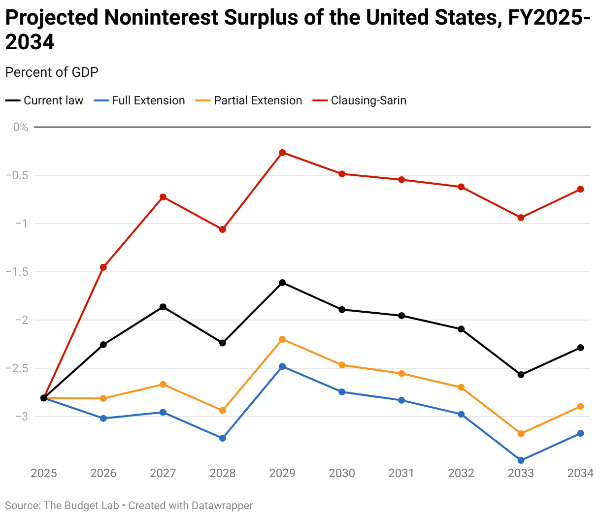
- We estimate that Full Extension would cost 0.9 percentage point of GDP on average over the next decade, increasing primary deficits by more than 40 percent over the decade.2 Fully extending the expiring individual income tax provisions of the TCJA would cost approximately $2.8 trillion dollars over the budget window. As a share of the overall economy, this revenue loss is largely stable in the longer run and remains at 0.8-0.9 percent of GDP through 2054.
- The Partial Extension scenario has an average annual budget cost over the decade of 0.6 percentage point of GDP. This scenario costs about $1.6 trillion over the budget window and reduces revenues by 0.4-0.5 percent of GDP in the longer run.
- The Clausing-Sarin reform cuts average annual primary deficits by nearly two-thirds. It raises 1.3 percentage points of GDP of new revenues on average over the decade. We estimate the proposal would raise a net $4.3 trillion over the budget window, with more substantial savings in subsequent years.
Behavioral feedback assumptions in the conventional scores
As described at the beginning of this section, our conventional scores for these three reform options reflect the budgetary impact of how taxpayers will respond to minimize tax liability under the new tax laws. Income shifting across business entity type is one such example. These reforms alter the relative tax differential between business income earned through a C corporation (which faces the corporate tax rate and eventually dividend or capital gains taxes) versus pass-through business income (which faces ordinary income tax rates and, in some cases, benefits from the QBI deduction). We expect the share of business activity organized in C-corporate form to fall under all three scenarios. Another example is charitable giving. By limiting the number of itemizers and lowering marginal tax rates, these reforms generally reduce the tax subsidy for giving; we project that taxpayers would respond by giving somewhat less, claiming fewer deductions, and thus raising tax revenue relative to baseline, all else equal.
In general, when it comes to behavioral feedback assumptions, we have largely attempted to mimic our understanding of how JCT, CBO, and Treasury’s Office of Tax Analysis (OTA) would address these issues. A full accounting of our methodological choices can be found in the Technical Appendix. However, we depart from government scorekeepers in two key areas that affect our Clausing-Sarin estimates.
The first is our assumed baseline capital gains elasticity value of -0.6. This elasticity is a departure from the elasticity presented by Dowd et al. (2015) of -0.72.3 Over the last few years, there has been an active academic discussion about the revenue-maximizing capital gains rate centered on this elasticity. Gravelle (2021) presents a thorough discussion of the research and revenue implications of behavioral responses. We feel that an elasticity of -0.6 best reflects that discussion. However, some recent econometric work suggests the elasticity may be even smaller, and some may prefer a smaller elasticity.4
Second, we project stronger net budget returns to IRS funding than CBO has done in the past. We understand the literature to suggest that there is a significant peer effect of increased audits that increases compliance. Traditionally, CBO has not included this indirect effect of deterrence in its projection of revenue related to increased IRS funding. However, a recent CBO report updates their methodology, and they now include deterrence effects.5 We expect subsequent CBO revenue estimates for this provision to be closer to our revenue estimates, but that remains to be seen.
Footnotes
Three provisions merit special consideration in this context. First, both the rate cut and QBI deduction line items reflect our expectation that if the deduction were extended, some businesses that would organize in the C-corporate legal form under current law would instead elect to be taxed as pass-through businesses. This kind of legal tax avoidance generates modest revenue losses in addition to the mechanical, or “static”, budget effects. Second, we assume that only half of net operating losses generated by the limitation on pass-through loss deductions are eventually claimed. Third, we assume that most states would continue to offer so-called “SALT cap workarounds” in the presence of a permanent limitation on the SALT deduction, and that owners of pass-through business would elect to employ these tax avoidance strategies at similar rates to those seen in recent years.
When calculating averages under the reform, we include years in which the policy reform is enacted only.
Dowd, Timothy, Robert McClelland, and Athiphat Muthitacharoen, . “New Evidence on the Tax Elasticity of Capital Gains,” National Tax Journal, 2015, 68 (3):511-44, https://EconPapers.repec.org/RePEc:ntj:journl:v:68:y:2015:i:3:p:511-544. For a discussion of the elasticity literature see Gravelle, Jane. “Capital Gains Tax Options: Behavioral Responses and Revenues.” CRS R41364, 2021. https://crsreports.congress.gov/product/pdf/R/R41364.
For instance, Agersnap and Zidar (2021) estimate a range of long-term elasticities between -0.5 and -0.3. Agersnap, Ole, and Owen Zidar. “The Tax Elasticity of Capital Gains and Revenue-Maximizing Rates.” American Economic Review: Insights, 2021, 3(4): 399-416.
Burke, Kathleen and Shannon Mok. . “How Changes in Funding for the IRS Affect Revenues.” Congressional Budget Office, February 2024, https://www.cbo.gov/publication/60037#_idTextAnchor006.