
The Inflationary Risks of Rising Federal Deficits and Debt
Key Takeaways
-
Higher debt adds to the risk of inflationary pressure in both the short- and the long-run, through aggregate demand, inflation expectations, crowding-out of private investment, and worries about fiscal dominance.
-
Even in countries where central banks have the tools to fight inflation with higher real interest rates, such as the United States, household cost-of-living still rises.
-
The conventional economic models we use show that in the short-run, a permanent primary deficit increase of 1% of GDP—roughly in line with the cost of fully extending the individual provisions of the Tax Cuts and Jobs Act—raises inflationary pressure after 5 years equivalent to a loss in household purchasing power of $300-1,250 per household in 2024$. (This is a subset of the total economic effect of higher debt.) A more unconventional model raises the possibility that the effect is even higher in the short-run. This effect alone is more than half the benefit of the policy itself.
-
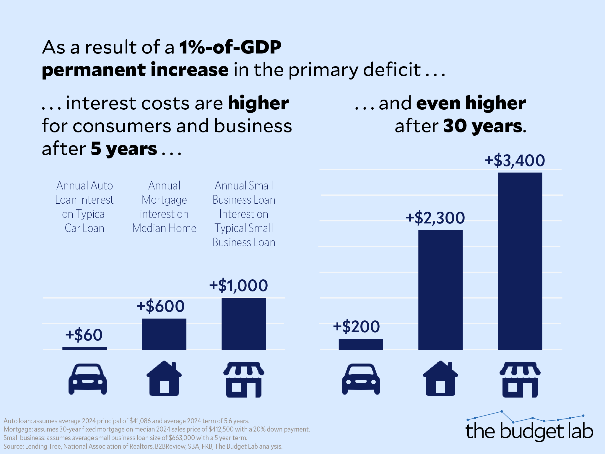
If the Federal Reserve reacts in the short-run, higher interest costs burden consumers and benefit savers. For example, the same 1% of GDP shock leads to higher mortgage interest payments equivalent to $600-1,240 per year in today’s housing market, and mortgage rates move in lockstep with the 10-year Treasury.
-
After 30 years, price pressures reach the equivalent of a $16,000 cumulative loss per household in 2024$. Mortgage rates are almost a percentage point higher, leading to $2,300-$2,500 higher interest payments in today’s market equivalent, and real household wealth declines by $24,000-36,000 per household on average in 2024$.
Introduction
Today, the United States faces an unsustainable debt trajectory. By end of the next 10 years, the Congressional Budget Office (CBO) projects America’s debt-to-GDP ratio will approach 120% under current law, surpassing the prior record reached in 1946 in the wake of World War II. If expiring tax policies are extended without offsetting deficit reduction, debt would end the decade even higher. Given this moment of heightened consumer price sensitivity and fiscal crossroads in the policy, the interplay between debt & deficits and inflationary pressures merits renewed scrutiny.
For decades, low and stable inflation has served as a bedrock of economic policy in advanced economies. This has been a long, hard-learned lesson. From the hyperinflation traumas of the Weimar Republic to the stagflation shocks of the 1970s to the global pandemic inflation, policymakers have been reminded time and again that price stability is not merely a technocratic objective on paper but a prerequisite for sustainable growth, equitable resource allocation, and public trust in economic institutions.
This paper argues that elevated federal debt increases the risk of inflationary pressure through several channels in both the short- and the long-term. Some are familiar and conventional mechanisms, such as short-run aggregate demand. Other channels include crowding-out of capacity investment, amplifying fiscal dominance concerns, and amplifying inflation expectations.
Overview: Why Low Inflation Remains a Policy Priority
At its core, inflation can act as a stealth tax on economic certainty. When prices rise unpredictably, households face a dual burden: first, the erosion of their nominal incomes, and second, heightened uncertainty about future purchasing power. Lower-income households bear these uncertainty costs disproportionately, as they allocate larger shares of their budgets to non-discretionary items like food and housing—categories less flexible for substitution and particularly vulnerable to supply shocks, though it is not clear that low-income households always bear more of the actual costs of inflation.
Equally corrosive is inflation’s impact on decision-making frameworks. When businesses and consumers cannot distinguish relative price changes from economy-wide trends, resource allocation grows inefficient. Firms delay investments, households hoard goods, and lenders demand higher risk premiums—a dynamic starkly visible during the 1970s “Great Inflation,” when annual U.S. PCE price growth averaged 6.6%, versus 2.2% over the 1960s.1 Research shows that higher inflation volatility can detract from growth, especially among countries with records of high inflation and low-credibility central banks.
Modern central banking in advanced countries has been shaped by the lessons of past inflationary crises. This evolution has taken many forms in the post-World War II decades, including the adoption of explicit inflation targeting or price stability frameworks, the gradual enshrining of political independence, and, more recently, the expansion of monetary policy toolkits to include unconventional actions like quantitative easing and forward guidance. As recently as 2023, all but six central banks globally explicitly prioritized low inflation, often codified in law. As discussed later, the rise of central bank credibility and anchored inflation expectations has shifted the trade-offs between debt and inflationary pressure.2
Literature Review: The Inflationary Channels of Elevated Federal Debt
The relationship between public debt and inflation has been a central macroeconomic debate for decades. This review synthesizes empirical and theoretical insights into short- and long-run mechanisms linking debt to inflation.
Short-Run Mechanisms: Demand Shocks, Supply Chains, and Central Bank Missteps
In the short-run, debt adds to pressure from the interplay of Keynesian demand dynamics and temporary supply-side constraints. The pandemic was only the latest example of this economic story. One global comparative study, Jordà and Nechio (2022), concluded that while both deficits and inflation rose globally during the pandemic, the marginal fiscal actions by the United States in 2020 and 2021 and their effects on demand accounted for 3 percentage points of inflation by the end of 2021, though other advanced economies’ cumulative pandemic inflation began catching up with the US in 2022. CEA (2023) concluded that while supply-side issues were a major inflationary driver in their own right, they also interacted with the extraordinary global fiscal impulse, heightening the direct inflationary effects of fiscal policy. These shocks fed into heightened inflation expectations among both households and businesses.
Long-Run Channels: Expectations Anchoring and Crowding-Out
Over extended horizons, debt sustainability hinges on inflation expectations and fiscal-monetary coordination. Elevated debt-to-GDP ratios amplify crowding-out risks in the neoclassical framework: the possibility that growing government debt ties up an ever-greater share of private capital over time, raising interest rates and reducing investment. CBO generally assumes each additional percentage point of debt-to-GDP adds 2 basis points to the US 10-year Treasury yield. While directionally this is a well-established finding in the economic literature, as a long-term effect the point estimate is highly uncertain. Moreover, other factors weigh on interest rates as well; some, like demography, have been otherwise putting downward pressure on them. A smaller capital stock over time leaves a country more vulnerable to future supply chain shocks, which can raise inflation volatility. This is a particular risk given the rising uncertainty around future climate events, which have the potential to cause substantial supply-side damage and add to price pressure.
In regimes without central bank credibility, debt levels influence inflation expectations through fiscal dominance channels as well. (Fiscal dominance is the risk that debt and deficits reach a point where the government and central bank can no longer control inflation.) When investors perceive fiscal unsustainability, they demand higher inflation premiums, particularly in economies with short-maturity debt structures. In advanced economies like the United States, such effects are muted due to stronger institutional credibility on the part of the central bank. Note, however, that even in the best-case scenario, this just means that in advanced economies the trade-off runs through higher interest rates rather than higher inflation. Hence, throughout this paper, we more precisely refer to the trade-off in the context of the United States in terms of inflationary pressure, since the Federal Reserve in practice has to impose a cost from inflationary pressures through raising interest rates.
Some economists worry that persistent unsustainable deficits elevate fiscal dominance risk even in advanced economies, if lawmakers start putting political pressure on central banks to keep interest rates low to contain debt service costs.
Emerging markets offer an opportunity to study the direct trade-off between debt and inflation, often without the institutional complexities of a strong central bank. Studies find that dollarized debt and inflation-targeting regime adoption critically moderate economic outcomes. Emerging markets without inflation targeting experience persistent expectation de-anchoring after debt shocks. High initial debt compounds these effects. The nature of the shock can also matter. For example, Valencia et al. (2023) demonstrates that supply-driven inflation shocks in EMs raise debt-to-GDP ratios by eroding primary balances and spiking borrowing costs, whereas demand-driven shocks (e.g., stimulus-fueled growth) can reduce debt burdens if expectations remain anchored. This asymmetry underscores the peril of fiscal dominance in low-credibility regimes.
Modeling Short-Run Effects
Estimating inflationary pressure from all of these various channels necessitates economic modeling. Different models of the economy at different horizons envision different mechanisms for debt to affect inflationary pressure and inflation. That’s because the relationship between public debt and inflation varies across economic paradigms. Please see the Appendix for a longer discussion.

The table above shows first how we would expect prices to evolve without a Federal Reserve response, and what that would mean for the purchasing power of household disposable income. Second and separately, it shows the cost in additional interest payments for mortgages if the Federal Reserve did respond. The simulations without a Federal Reserve shock show the result of an increase in the deficit and debt from a permanent 1%-of-GDP increase in federal transfers, without any reaction from the Federal Reserve. We chose a generic transfers shock because it would minimize any longer-run change in substitution effects and economic incentives resulting from federal policy (think of this shock as being equivalent to an on-going lump sum subsidy of ~$1,000 per adult per year in 2024$). This is not substantially different in magnitude from the effect of extending the individual provisions of the TCJA, whose cost through 2035 averages to an increase in debt-to-GDP of slightly more than 1 percentage point a year against current law. This is the appropriate way to model gross inflationary pressure from a fiscal shock. The shock boosts aggregate demand and, without intervention from the Fed, causes a feedback loop between actual inflation, inflation expectations, and wage growth. Note that the household income effects we report in the table above are equivalent inflationary or interest rate effects in isolation; they do not incorporate the broader negative economic effects of debt on real income nor do they include the positive effects of our illustrative policy.
Inflationary/Price Pressure Trade-Off
While the models have different results, all of them show a rise in prices without Federal Reserve intervention. For instance, Figure 1 below shows FRB/US (the Federal Reserve’s workhorse macroeconomic model) with core PCE prices at roughly 0.2 percentage points higher five years out. Think of this as the cumulative inflation effect over the first five years. As seen earlier in Table 1, one way to conceptualize the loss in consumer welfare from price increases is that it would be equivalent to average household disposable income being $330 lower per household per year in 2024$—note that this is separate from the positive income effects of the policy itself, which here is purely a mechanism chosen for rising debt.

MA/US—a private-sector model similar in structure to FRB/US—suggests a deeper inflationary cost from debt than FRB/US does. That’s because inflation in MA/US is less inertial than in FRB/US: by the end of five year, the fiscal shock has caused the core PCE price level to be 0.76% higher—equivalent to a loss in disposable income of $1,250 per household in 2024$ as seen in Table 1—and annual core PCE inflation is running 0.3 percentage points higher by the end of the five-year window.

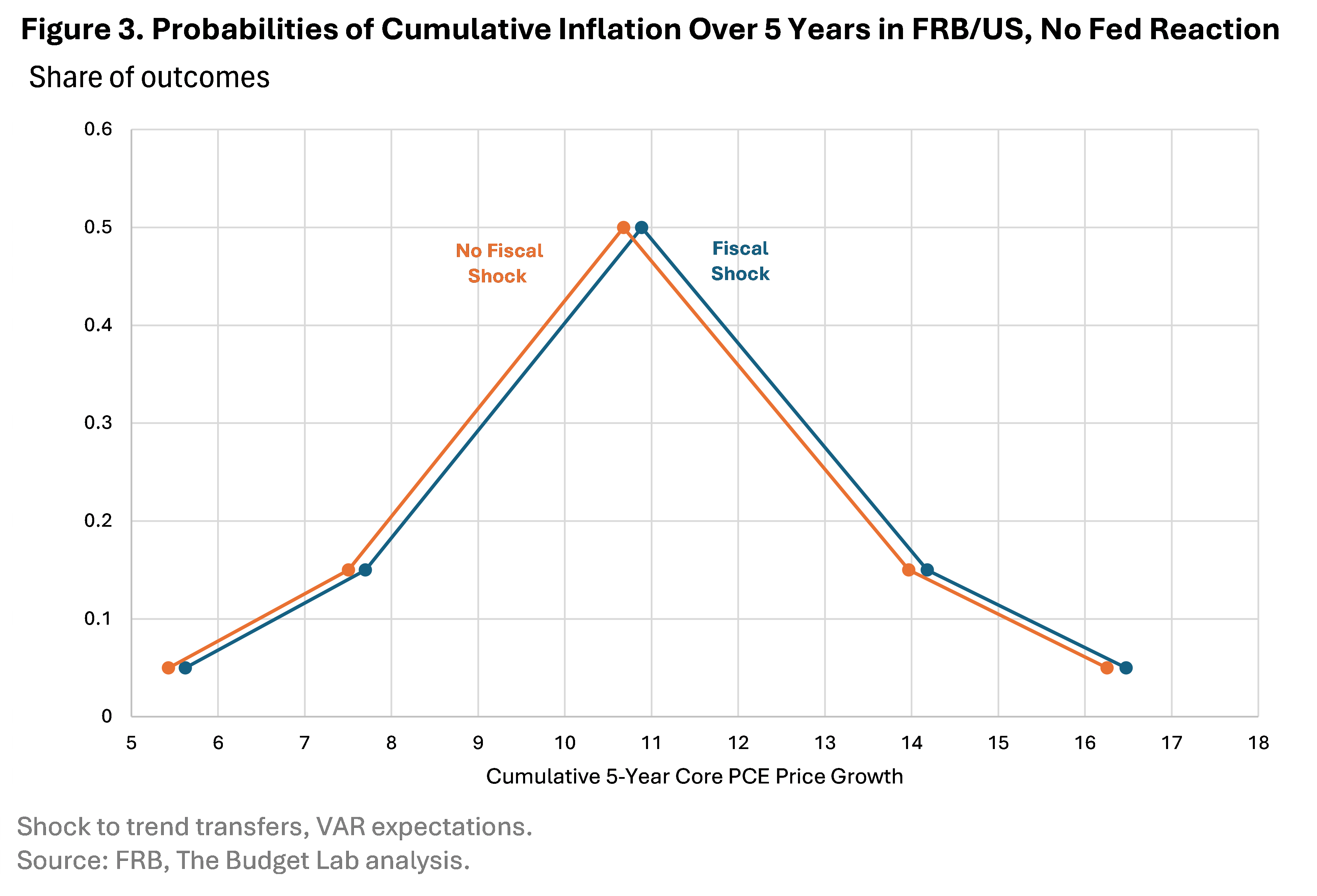
We can also look at how the probability risks around short-run inflation change with greater debt. By running FRB/US thousands of times with random historical shocks, we can examining the range of outcomes and produce a distribution. Figure 3 below shows how the 5-year inflation risk curve shifts under our illustrative fiscal shock, again without Fed intervention like the first FRB/US simulation. As you can see, the entire curve shifts, not just the median outcome, but outcomes under both good and bad surprises. The median outcome without a fiscal shock is cumulative 5-year inflation of just over 10.5% (a bit over 2% inflation per year on average); with the fiscal shock, the median shifts higher (to the right) by the same 0.2 percentage points we found in the first exercise. The 5%-low-probability outcome is roughly 5.5% cumulative inflation (just over 1% a year on average), while the 5%-high-probability outcome is over 16% inflation (over 3% a year on average); both shift higher as a result of higher debt.
FRB/US and MA/US are large structural models that take a Keynesian lens to debt shocks in the short-run. What about other short-run perspectives? One is the Fiscal Theory of the Price Level (FTPL), which holds that market participants have perfect foresight into the future and gradually adjust prices in an economy so that the current stock of inflation-adjusted debt is equal to the expected value of future primary surpluses. In the FTPL context, a permanent shock to the deficit of 1% of GDP both increases debt on an ongoing basis and decreases the net present value of primary surpluses. Actors in our toy FTPL model continuously update their expectations as they see the higher deficits persist. This leads to a much larger price level effect than in FRB/US or MA/US: five years out, prices are more than 9% higher after adjustment (see Figure 4 below), an almost-$15,000 loss for the average household in 2024$ as seen earlier in Table 1.

Other models are more purely empirical. Under a pure demand-side simulation in Bernanke & Blanchard’s 2023 model (BB2023), where we assume no supply-shortage response—the price level is 0.25% higher after five years (see Figure 5), higher than the FRB/US response but a bit below MA/US. This is the equivalent of a loss of $400 per household in 2024$ as seen earlier in Table 1. We also show the price response under an illustrative scenario where the shock also prompts a temporary supply shortage: in this case, the BB2023 measure of shortages rises to 20% of its maximum for a full year before returning to normal.3 This shows what the price response might look like if supply were endogenous to the demand shock. As you can see in Figure 5, prices rise far more, by roughly 0.9% after five years in response to the debt shock, a $1,500-per-household loss on average (Table 1).

Running a similar simulation in the Ball, Leigh, & Mishra (2022) model show a price level that is 0.55% higher after five years (Figure 6), the equivalent of a $900 per household loss on average in 2024$ (Table 1).

Interest Rate Trade-Off
Of course, in reality, as the Fed tightens monetary policy in reaction to heightened inflationary pressure, the trade-off shows up more in the form of higher interest rates and less in the form of realized inflation. To show how the debt-inflation trade-off often actually operates in the US in the short-run, we repeat the same exercise, but allow the Federal Reserve to react immediately in a manner prescribed by a classic Taylor Rule. In FRB/US, the effect to inflation is now imperceptible—mere basis points—and even after five years the price level is only 0.05% higher (Figure 7).
But debt-financing still comes with costs. Now, short-run interest rates are persistently higher, by about 0.25%. This has reverberations throughout different types of consumer products. Mortgage rates are 23 basis points higher after five years, which, in today’s housing market, would add about $600 per year in interest payments to the median home. For the average auto loan on a new car, this would be the equivalent of $60 a year in extra interest.4 For the average small business loan, that means an extra $1,000 in interest annually.5 Meanwhile, real household wealth falls by 1.2% over 5 years (Figure 7), the equivalent of a $14,000 loss on average today (Table 1). And even within the five years, the capital stock begins to take damage from higher interests and crowding-out. So even with a credible central bank, households still face a cost-of-living tradeoff from higher debt even in the short-run, just through interest costs rather than prices. Meanwhile, in MA/US, mortgage rates are 47 basis points higher at the end of five years—the equivalent of an extra $1,240 in interest payments annually in today’s market.

Long-Run Modeling
We also look at the long-run impacts of a fiscal shock. As Figure 8 below shows, in a Solow Growth model (whose parameters are explained in the appendix), over 50 years the capital stock is more than 10% smaller, and real output is more than 3% lower.

We can also return to the FRB/US model, where we find that price pressures grow over time in the wake of the debt shock, reaching the equivalent of an-almost 10% higher price level after 30 years (Figure 9), the equivalent of a more-than-$16,000 loss in 2024$ per household (Table 1). Higher debt crowds out private investment, raising interest rates, lowering the capital stock, and depressing income. Three decades out, the private capital stock is 4% lower—a smaller effect than our Solow growth simulation but still substantial—and real gross national product is more than a full percentage point lower. That’s the equivalent of $4,000 per household less by 2055 in 2024$. Real household wealth is 2% smaller, a $24,000 loss in 2024$. Everyday interest rates rise as debt puts upward pressure on benchmark yields: conventional mortgage rates, for example, are 85 basis points higher in 30 years (in today’s context, that would add roughly $2,300 per year to the interest payment on the median-priced house). New car loan interest on the average 2025 loan would rise by $200 per year, and interest on the average 2025 small business loan would rise by $3,400 annually.

If we run the model using the 10% capital stock decline in our earlier Solow growth simulation, price pressure over 30 years from our debt shock is roughly the same at almost 10 percent, however other economic outcomes are more dire. In particular, real income declines are doubled, with real GNP per household $8,000 smaller on average in 2024$ (Figure 10). Mortgage rates are 95 basis points higher—the equivalent of $2,500 extra per year in interest payments today—and real household wealth is now 3% smaller, or $36,000 per household in 2024$ on average.

Nonlinearity Considerations
A final note is that the relationship between government debt and economic outcomes, including inflationary pressure, is complex and uncertain in the long-run. A key risk with debt is nonlinearities—the dynamic wherein linear increases in primary deficits lead to macroeconomic and debt outcomes that spiral out of control. There are a few mechanisms that might drive this.
One is just the intersection of crowding-out and the basic math of r – g (the difference between interest rates and economic growth). At r = g, primary balance keeps debt-to-GDP stable over time. But if interest rates suddenly rise above growth rates for some reason, debt suddenly shifts to an unsustainable, convex trajectory even if the government runs a primary balance. And if interest rates rise because the government is not running a primary balance but is already starting from an unsustainable trajectory, then the feedback from interest rates to deficits to debt and back to interest rates can lead to a debt outlook that explodes over the long-term. Many of the models used in this analysis—such as FRB/US and the Solow growth model—capture the nonlinearities associated with interest rate feedback.
A related possible nonlinearity is that there are threshold effects associated with debt. At low to moderate debt levels, increases in government debt may have limited impact on inflationary pressure and interest rates. However, once debt surpasses a certain threshold, further increases may lead to more pronounced inflationary pressures. This possibility suggests that the impact of debt on inflationary pressure is not constant but rather depends critically on the existing debt stock. Countries with already high debt levels may find that additional borrowing has outsized effects on inflation expectations and realized inflation. The existence of threshold effects for sovereign debt is hotly debated in public finance. Even researchers that agree on their relevance disagree on where the threshold lies or whether it applies to large advanced economies like the United States.6
Conclusion
The relationship between government debt and inflationary pressure is complex and multifaceted, with both short-term and long-term implications for economic stability and growth. The various models and simulations presented in this paper demonstrate that elevated federal debt can increase the risk of inflationary pressure through several channels, including direct demand effects, expectations feedback, reduced capacity and capital stock, and potential fiscal dominance concerns. While the magnitude of these effects varies across different models and time horizons, the consistent message is that persistent high levels of government debt can have significant consequences for price stability, interest rates, and overall economic performance.
The analysis also highlights the critical role of central bank credibility and fiscal-monetary coordination in mitigating the inflationary risks associated with high debt levels. As demonstrated by the FRB/US model simulations with Federal Reserve reaction, a credible monetary policy can help contain short-term inflationary pressures. But this still comes at the cost of higher interest rates. Moreover, the long-run simulations underscore the potential for substantial negative effects on capital accumulation, output, and living standards if debt levels continue to rise unchecked. These findings emphasize the importance of prudent fiscal management and the need for policymakers to carefully consider the long-term consequences of persistent deficit spending, particularly as the U.S. debt-to-GDP ratio approaches historic highs.
Modeling Appendix
FRB/US is the Federal Reserve’s workhorse macroeconomic model. It’s a large-scale structural model with nearly 400 equations and identities. Its short-run properties are built around a New Keynesian Phillips Curve where wage and price formation are estimated simultaneously. The model allows for both adaptive (backwards-looking) and rational (model-consistent) expectations. As a Federal Reserve model, the focus of FRB/US is monetary policy, not fiscal policy, but the model does include summary variables to capture high level categories of federal spending, revenues, and federal debt. As mentioned earlier, we modify the FRB/US equations to add a channel whereby growing debt affects interest rates in line with Congressional Budget Office assumptions. Specifically, this analysis modifies the FRB/US equations for the Treasury term premia so that the 10-year premium rises by 2 basis points for every percentage point debt-to-GDP rises above the FRB/US baseline. Note that our FRB/US simulations are not official forecasts or exercises of the Federal Reserve Board. In FRB/US, inflation is highly inertial—meaning that the model assumes structurally that inflation can only change gradually—and also assumes that inflation expectations are well-anchored around the Fed’s 2% inflation target.
MA/US
MA/US, developed by Macroadvisers and now maintained by S&P Global, is a large structural macroeconomic model of the same class as FRB/US. MA/US has even more detail about federal fiscal outcomes than FRB/US which gives it a broader focus than just monetary policy.
The Fiscal Theory of the Price Level (FTPL)
Unlike FRB/US and MA/US, FTPL is not a “commercial model” but rather a theoretical class of model, and one that makes some significantly different assumptions than those underpinning Keynesian models. FTPL holds that the price level adjusts to equilibrate the current stock of real debt with the net present value of expected future primary surpluses. Put another way:
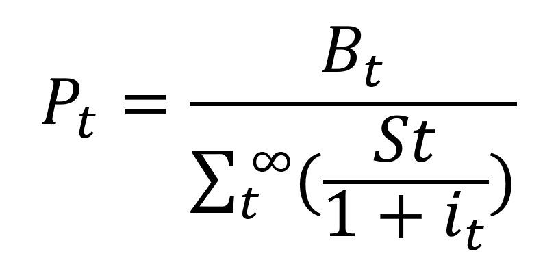
where P is the price level, B is the stock of federal debt, S is the primary surplus, and i is the interest rate.
In words: FTPL holds that bond holders are rational with perfect foresight. If an unsustainable debt shock occurs—one where the expectation is that the government will not eventually offset the shock with higher taxes or lower spending—then inflation adjusts immediately.
To simulate what FTPL implies for inflation, we build a “toy” FTPL model based on the latest CBO long-term outlook of primary deficits, debt, and interest rates.
Bernanke & Blanchard (2023)
Olivier Blanchard and Ben Bernanke (hereafter BB2023) published a widely-cited analysis of the pandemic rise in inflation using an empirical, short-run dynamic model. It is essentially a reduced-form VAR that incorporates inflation, wage growth, slack, trend productivity, short- and long-run inflation expectations, and supply shortages. The model is estimated on pre-pandemic data, and prices are in terms of headline CPI.
BB2023 has more detail than the FTPL model, but is still tiny in scale compared to FRB/US and MA/US. Most challengingly, BB2023 has no direct fiscal module. It also does not have an explicit central bank, though Fed reactions are implicit in the model’s estimated coefficients.
Nevertheless, we can still simulate an illustrative short-run fiscal shock in BB2023 with some upfront calibration. The channel for the shock to affect inflation is the conventional Phillips Curve channel of labor market slack, which in BB2023 is measured by the vacancy-unemployment ratio (V/U). In FRB/US, our 1%-of-GDP fiscal shock translated into a 1% higher real GDP level in the short-run, a multiplier of 1, which makes sense in the context of our exercise where we are explicitly modeling no Federal Reserve reaction. Therefore, we need to calibrate the V/U shock in BB2023 that would be consistent with 1% higher real GDP growth. In unemployment space, this calibration is done using a rule-of-thumb called the Okun Ratio (typically assumed to be 2), but there is no such conventional assumption that we are aware of for the V/U ratio, so we need to estimate one. We run a linear regression over 2006-19 of the Q4-Q4 change in the V/U ratio on the change in log real GDP. In this specification, the intercept represents trend GDP growth over this period, and the coefficient on the change in V/U represents the “V/U Okun” ratio. This yields a factor of 7.4. So the V/U shock associated with a 1 percentage point increase in real GDP is 1/7.4 or .135.
Ball, Leigh, & Mishra (2022)
The model from Ball, Leigh, & Mishra (2022) (hereafter Ball2022) is, like BB2023, an empirical model that incorporates V/U. Unlike BB2023, the model is a cross-sectional, single-equation Phillips Curve model, and allows for nonlinearities in V/U. So while Ball2022 leaves outs BB2023’s explicit channels for expectations, shortages, and wages, it probably does capture some of these relationships in its nonlinear structure. Prices in Ball2022 are expressed in terms of median CPI.
We run the same BB2023 shock through Ball2022. Since starting levels matter in a nonlinear model like Ball2022, we assume an equilibrium V/U ratio of 1.2, the 2019 average.
Long-run Modeling
Using the Solow Growth Model to Think About the Capital Stock
The Solow Growth Model, developed by and named after Robert Solow, is one of the foremost models used in modern economic growth theory. The model provides a framework for analyzing long-term growth based on the contributions of capital accumulation, savings, depreciation, labor force growth, and technological progress. The Solow model demonstrates how these factors interact to determine an economy's output and how they influence the path towards a steady state of growth.
As a long-run neoclassical model concerned primarily with changes to equilibrium paths, inflation and inflationary pressure is not a standard variable tracked by the model. However, it can analyze dynamic important to long-run inflation risk, such as investment and the capital stock. In the exercise following, we use our Solow results as a long-run input into FRB/US.
We initialize our Solow model using conventional parameters. We assume a labor force growth rate of 1%, a labor productivity growth rate of 1.5%, a depreciation rate of 5%, a savings rate of 3%, a capital share of 0.3, and a TFP coefficient of 1. However, the canonical Solow Growth Model does not include a module for government debt. We therefore add simple mechanisms for debt to affect investment in the model, calibrated to CBO assumptions. We assume a baseline where the interest rate r equals the steady state growth rate of output g. Debt-to-GDP evolves based on r, g, and the primary deficit-to-GDP p. In response to a primary deficit shock, r rises and investment gets crowded out. We assume that r goes up 2 basis points for every percentage point debt-to-GDP above baseline, and that investment falls $0.33 for every dollar increase in the annual deficit. Our modified Solow model is thus able to show how the capital-output ratio adjusts to a 1%-of-GDP permanent primary deficit shock.
An important detail to note is that in reality, the nature of the debt shock matters in the long-run. Here, we are simulating a generic debt shock which solely has crowd-out effects on private investment, to isolate the debt effect. Debt-financed policies however may have countervailing positive effects on the capital stock and labor supply over time, such as infrastructure spending or effective childhood interventions – or in the case of a recession.
Modified FRB/US
We turn back to FRB/US here. In the short-run, FRB/US is a Keynesian demand-driven model, but in the longer-run it is more neoclassical in the vein of the Solow growth model, where capital accumulation, population growth, savings, and productivity are more important.
We run long-run simulation two ways: with the permanent 1%-of-GDP deficit shock estimates entirely in-model, and with the capital stock effect calibrated to the Solow growth exercise discussed in the previous section. We show “price pressures” as the price level effect ex. Federal Reserve response, but the other economic effects assume the natural rate adjusts over time in the model and that the Federal Reserve shifts the stance of policy in response.
Footnotes
- Annualized average inflation measured over the 40 quarters of 1969 Q4-1979 Q4.
- One important asterisk is that inflation benefits debtors (since debt is typically nominal), including the federal government. An increase in the central bank inflation target mechanically leads to a one-time price level shift that reduces debt-to-GDP. However, this may come at the cost of central bank credibility and inflation volatility.
- This 20% assumption is calibrated based on our V/U shock as a share of the total rise in V/U from 2019 to its peak during the pandemic.
- Assuming a $41,086 principal on a 5.6 year loan.
- Assuming $663,000 in principal on a 5 year loan.
- See Salmon (2021) for a good literature review.