Modeling the Revenue and Distributional Implications of a Value Added Tax
By their very nature, indirect taxes (like excise taxes or value added taxes) reduce the real value of income earned through working and, in some cases, investing. This effect carries two major implications for budgetary scorekeeping analyses of indirect tax proposals:
- Additional revenue effects. Because other taxes are based on income (like individual and corporate income taxes) and the real value of income falls in response to an increase in indirect taxes, the real value of other taxes also falls. This second-order revenue loss is known as an “offset” and is crucial for understanding the broader budgetary impact of indirect taxes.
- Distributional effects. Indirect taxes affect labor, capital, and transfer incomes differently—differences which determine who ultimately bears the economic burden of indirect taxes.
In this report, we use the case of a value added tax to illustrate how we estimate the budgetary and distribution effects of broad-based indirect tax proposals.
Background
Taxes are often categorized as being either direct or indirect. The exact delineation between these groups is famously blurry—disagreements date back at least five decades—but one common definition is as follows: direct taxes are levied on the net income of an individual or business, while indirect taxes are assessed on the production or sales of goods and services. In this understanding, direct taxes include the individual income tax (which taxes the labor, business, and investment income of families) and the corporate income tax (which taxes the profits of corporations); excise taxes, sales taxes, value added taxes (VAT), and tariffs are examples of indirect taxes.
A key feature of indirect taxes is that they are applied at the firm level but do not allow a deduction for the cost of labor, a design which mechanically creates a wedge between the amount paid by final consumers and the funds available to compensate the factors of production. This wedge carries an implication: either consumer prices rise or nominal incomes fall.1 Put differently, indirect taxes are either “passed forward” to consumers or “passed back” to incomes.2
Whether prices rise or nominal incomes fall is a policy choice made by the Federal Reserve. Abstracting from transition effects, these scenarios are identical in inflation-adjusted terms: either nominal incomes fall, or the real purchasing power of those incomes falls.3 For small changes in excise taxes, the economy-wide impact on consumer prices would be small enough such that the Fed would likely maintain its inflation target, meaning that nominal incomes would fall slightly. For large increases, however, it is likely that the Fed would “look through” the policy change and temporarily ease policy, allowing for a one-time increase in the price level rather than forcing nominal wage cuts across the economy. Indeed, international experience with VATs suggests this outcome is likely.4
Revenue Effects
When incomes change—as is the case in response to indirect taxes—so do taxes that are based on income. Consider the introduction of a new indirect tax. If the Federal Reserve holds the price level fixed and nominal incomes fall, the bases for taxes such as individual and corporate income taxes will fall. If instead prices are allowed to rise, the real value of tax receipts—the quantity of goods and services the government can purchase per dollar of revenue—is lower. In either case, an increase in indirect taxes causes an offsetting decrease in revenues elsewhere, meaning that the government raises less than one dollar per new dollar of indirect taxes.
Official scorekeepers account for this budgetary “offset” by estimating the effective marginal tax rate on different factor income categories then scaling any first-order indirect tax revenue changes by one minus the total rate. The Joint Committee on Taxation (JCT) currently estimates that the offset is generally about 24 cents—that is, one dollar of new indirect tax revenue leads to about 76 cents of net government revenue.5 This approach can be interpreted as reflecting the pass-backward scenario.
Distributional Effects
Indirect taxes affect different types of income—and thus taxpayers—differently. In the case of a new broad-based value added tax, the extent to which a taxpayer is burdened depends on several factors:
- The economic character of their market income. Labor income falls in real terms regardless of whether prices rise or nominal incomes fall. Capital income attributable to investments made prior to the tax increase is generally burdened, as income available to pay creditors and owners is either lower (pass-backward) or the real value of these nominal income streams is lower (pass-forward). For investments made after the introduction of the tax, when nominal rates of return are renegotiated to account for the higher price level, only above-market (“supernormal”) returns are burdened.
- How much wealth they own. If prices rise, the amount of goods and services that can be consumed by spending down existing net worth falls in real terms; if prices are held fixed, then nominal asset prices would fall to reflect lower nominal future cash flows. Some of this burden is avoided if only a fraction of wealth is eventually consumed and the rest is bequeathed to heirs or charity.
- To what extent taxes and transfers are indexed to inflation. If taxes and transfers are indexed to inflation, then indirect taxes have no effect on the real value of net transfers (either net transfer income rises with the price level or the nominal value of transfers and consumption are unchanged). If taxes and transfers are instead not indexed to inflation, then a pass-forward scenario leaves transfer recipients worse off in real terms. Social Security is a special case due to its pension-like qualities. In the pass-forward scenario, Social Security benefits are unchanged for current retirees due to the cost-of-living adjustment, but future benefits for current workers are not scaled up to offset the higher price level because nominal wages are unchanged. The pass-backward scenario is economically equivalent: current retirees are unaffected, but nominal wages cuts generate smaller future benefits for current workers.
- The progressivity of the taxes and transfers. As per the discussion of the revenue offset above, a real decline in incomes implies a real decline in taxes. This lower tax burden is a real benefit which partially offsets the loss of income caused by the indirect tax hike. The size of this offset and its distribution by income depends on the current-law distribution of taxes.
A complete theoretical account of these dynamics can be found in Toder et al. (2011), Burman et al. (2006), and this 1992 CBO study.
How We Model Value Added Taxes
Our methodological strategy is based on (a) the existing infrastructure of our tax microsimulation model and (b) the approximate economic equivalence of the pass-forward and pass-backward scenarios. At a high level, our approach is to:
- Estimate the first-order revenue effects of the indirect tax change. These revenue projections are estimated “off-model”.
- Assume that the tax is passed forward and run the model. Presented with a change in indirect taxes, the tax microsimulation updates its projection of the price level and makes corresponding adjustments to indexed tax parameters, Social Security benefits, and capital income.
- Express tax model output in baseline dollars. Direct taxes are re-calculated using these new projections. The resulting revenue projections are deflated by the price level change such that any revenue effect is expressed in baseline dollars, allowing for a comparison which is consistent with scorekeeping convention. Real income changes at the micro-level are incorporated into distribution tables.
We believe this approach confers several benefits, one of which is micro-level realism. By using a “ground up” approach, we can specify the exact dynamics which give rise to the aggregate-level revenue offset and incidence results. Another benefit is its relative simplicity of implementation: the pass-backward scenario would involve a more complicated series of adjustments to nominal incomes. And because we can deflate the results to baseline dollars, a third benefit of our approach is its flexibility to approximate both the pass-forward scenario (with its pollical-economy feasibility) and the pass-backward scenario (which maintains a fixed price level as per scorekeeping convention).
In this section, we describe our approach in further detail using the case of a 10 percent VAT as a motivating example.
Estimating the First-order Revenue Effects
To estimate the gross revenue raised under a VAT, we start with total personal consumption expenditures (PCE) and adjust the tax base to match that of a specific proposal. Common adjustments to PCE to arrive at a proposed VAT base include the removal of imputed consumption (such as certain financial services), the adjustment of housing to be on a gross investment basis rather than a consumption-flow basis, and other exclusions for certain categories, like health or education spending. The size of a given adjustment is based on recent historical averages of category shares of total PCE, which itself is assumed to grow with projected GDP.
For the exercise below, which is not concerned with a specific VAT base but rather how other revenues change in response to indirect tax changes, we simply assume that a non-specified 50 percent of PCE is subject to the VAT, taxed at a 10 percent rate.
Calculating the Price Level Effect
Indirect taxes create a wedge between factor prices and market prices. In the pass-forward scenario, market prices rise by the amount of the tax. In practice, however, there is no single “price level” but rather several indexes which measure the price of different bundles of goods and services.
For our purposes, we care about two broad categories of price indexes. The first are indexes which measure the price of personal consumption, including the CPI, chained CPI, and the PCE deflator. These indexes serve two purposes: first, because they are a suitable measure for understanding how household living standards change, we can use them to calculate real income changes for distribution tables; and second, chained CPI is the current-law tax code indexation metric. To calculate the level shift attributable to the introduction of a VAT, the projected VAT liability is divided by projected PCE. In our example, the price level effect for a 10 percent VAT on 50 percent of PCE generates a price level increase of 5 percent.
The other relevant index is GDP deflator, a measure of the price of all components of GDP, not just consumption. When expressing VAT-scenario revenues in baseline dollars, we require an answer to the question: what is the relevant price level from the government’s perspective? While not an especially well-defined question (especially when compared with the price level for consumers), one reasonable answer is that the government should principally care about GDP as a whole. As such, when calculating the real revenue raised by a VAT in the pass-forward scenario, we deflate counterfactual scenario revenues by the change in GDP deflator, calculated as VAT liability over GDP. In our example, the GDP deflator price level effect is about 3.4 percent.
In the tax microsimulation model, the new consumer price level feeds through into the module which projects the value of inflation-indexed tax parameters. In the case of a VAT, for example, tax brackets would be higher, the standard deduction would be larger, and so on—changes which reflect the tax code’s attempt to hold real tax liability constant across different price levels. Note that the maximum taxable earnings limit for Social Security payroll taxes would not be updated in this scenario, as only the consumer price level, not the wage level, would rise.
Updating Incomes
As discussed above, some forms of income would rise with the overall price level in the pass-forward scenario. The first such example is Social Security benefits, which would rise for current retirees but stay unchanged for future retirees. In Tax-Simulator, we first impute benefit claiming age for all records with Social Security benefits. Then, we scale up benefits by the cumulative excess consumer price inflation in the years since retirement. The effect of this logic is that, in the year following the introduction of a VAT, all Social Security income is scaled up such that there is no real decline in benefits. But as time goes on, the share of total benefits receiving a cost-of-living adjustment falls, as more and more current-period recipients retired after the VAT was enacted and thus receive no adjustment.
Investment income is the other major category of income that requires adjustment for VAT-driven price level changes. The size of the adjustment varies along two dimensions: new capital vs old capital, and normal returns vs supernormal returns. Nominal returns to new capital, which are not burdened by the VAT, rise with the price level increase; returns to old capital do not. Of returns to new capital, some fraction—assumed to be 50 percent in our model—represents the normal return, which rises with the price level; the remaining supernormal portion, burdened by the VAT, does not rise.
How investment income is allocated between new/old and normal/supernormal depends on the financing structure. For net interest income (i.e. returns to debt finance), we impute the share of returns accruing from debt issued after each year—the debt’s “vintage”—based on the maturity structure of marketable Treasury security in 2024.6 All debt is assumed to earn the normal return. Thus, in the context of a new VAT, the adjustment factor for net interest income for a given year is the cumulative excess consumer price inflation multiplied by the share of income attributable to debt issued after VAT enactment.
For capital gains and dividends (i.e. returns to equity finance), we impute the share of returns attributable to new investment by assuming a 5.7 percent economic depreciation rate. The equity return adjustment, then, is 50 percent (the share of income assumed to reflect supernormal returns) of the cumulative excess consumer price inflation multiplied by the share of income attributable to capital installed after VAT enactment. For pass-through income, we assume that 20 percent of net income represents the returns to capital (the other 80 percent being labor) and scale this component by the equity return adjustment.
The code implementing these adjustments can be found in economy.R.
Measuring the Budgetary Offset
After making all adjustments for price level changes, taxes are calculated at the micro level then aggregated to produce revenue projections. Three sets of revenue estimates are generated: nominal, real (i.e. deflated by the increase in GDP deflator), and share-of-GDP. The table below shows these metrics for fiscal years 2025 and 2026 under the VAT experiment previously described (i.e. a 10 percent VAT on 50 percent of PCE).
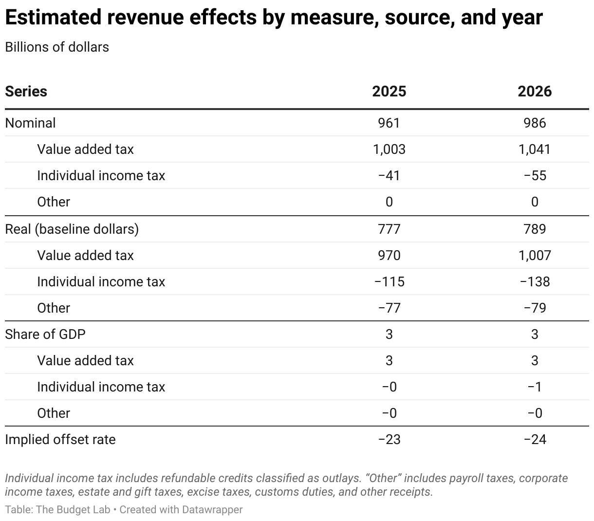
In nominal terms, gross VAT revenue is estimated to be about $1 trillion in 2025. Nominal individual income tax receipts fall relative to baseline due to tax cuts generated by inflation indexing. In real terms, however, estimated total revenue raised under the reform is less than $800 billion due to lower real other taxes. We estimate that real net revenue raised from a VAT would be about 76 to 77 percent of nominal gross revenues, suggesting an offset rate similar to that of JCT. This result points to the approximate economic equivalence of the pass-forward and pass-backward scenarios.
Note that a higher price level would affect non-revenue components of the federal budget as well. Transfers indexed to inflation would rise and purchases of certain goods and services would be more expensive. We do not currently incorporate these effects into our scores.
Calculating Distributional Effects
Tax-Simulator calculates various distribution metrics by comparing tax liability under baseline with tax liability under the reform scenario, then calculating averages across some dimension like income or ages. In the case of a VAT, however, tax burden takes the form of lower real incomes, not changes in liability. To calculate the distributional effects of a VAT, we simply compare after-tax incomes under the baseline with “real” after-tax incomes under the reform—that is, figures expressed in baseline dollars. This adjustment allows us to capture both the diminished purchasing power of incomes and any reduction in real tax liability.
The impact of a VAT varies by composition of income and by time since enactment. The figure below decomposes our estimated distributional effects of the 10 percent VAT, both in the year following enactment and in the 10th and 30th years of enactment.
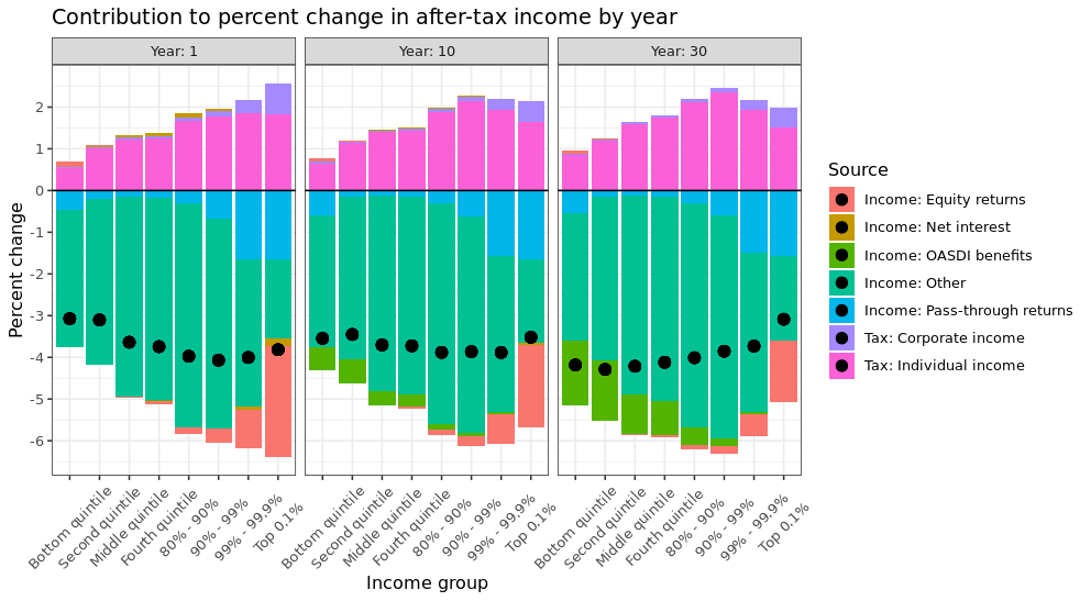
In the first year, the VAT is modestly progressive by this metric. Many lower-income tax units are Social Security recipients, which is indexed to inflation for current retirees and is thus unaffected by the VAT’s price increases. On the flip side, in the period immediately following the introduction of a VAT, all investment income—which disproportionately accrues to high-income tax units—is attributable to “old” capital and is thus burdened by the tax.
In the long run, however, the VAT’s distributional impact turns modestly regressive. A much smaller share of Social Security benefits receive the COLA adjustment for the VAT, as most retirees started claiming benefits after its enactment. In addition, returns to capital income are higher by this point because a larger fraction of income is attributable to investments made after the VAT was introduced.
These results are in line with those of other researchers, who find that a VAT’s distributional impact during the “transition” period is more progressive than when it is fully phased in. Note that the estimated long-run distributional effects are sensitive to the assumed share of supernormal returns. If supernormal returns are assumed to comprise a larger fraction of total returns to capital, then a VAT is more progressive. Also note that relative regressivity depends on the chosen tax base. A base that exempts goods and services disproportionately consumed by lower-income households will be more progressive, all else equal.
Potential shortcomings of our distribution tables are related to the following factors:
- Consumption bundle differences. Our approach is designed to model the effects of a broad-based VAT. But experience from other countries (and from state and local retail sales taxes) suggests that political economy factors may cause policymakers to exempt certain goods or services. Because the consumption share of specific goods and services varies with income, our approach may produce biased estimates of narrow-based VAT proposals.
- Lifetime consumption patterns. By measuring the burden of a VAT as the real decline in purchasing power of income, we are implicitly assuming that all income is eventually consumed. But some accumulated resources (i.e., savings plus capital gains) are given to charity or heirs, and this fraction generally rises with income. In either case, the burden is transferred to those who are gifted or inherit the money, and the assumption holds if the value of gifts or bequests is viewed as having consumption value.
- Cross-sectional vs lifecycle perspective. One simple alternative distributional approach would be to distribute aggregate VAT liability to income groups in proportion to their consumption. On a point-in-time basis, lower-income families consume a higher share of their cash income compared with higher-income families – with consumption rates often in excess of 100% of income (financed by borrowing or personal transfers). This approach, which is more interpretable on a cross-sectional basis, would generate more regressive results by construction. But it would fail to account for the longer-run economic dynamics described above. This tradeoff is a specific case of a more general conceptual difficulty in distribution analysis – how to incorporate economic changes accruing over a longer period of time in the context of a cross-section of the income distribution. See Burman et al (2006) for a deeper discussion on this topic.
- Asset price effects. We do not distribute the VAT burden associated with falling real asset prices. Data limitations prevent us from capturing this component at the current moment. In theory, this effect could be distributed either as a one-time effect placed on owners in the first year of enactment, or on an accrual basis using projections of when pre-enactment wealth is consumed. In either case, its exclusion biases our results in the direction of regressivity and once again highlights the conceptual issues surrounding the convention of distributing tax burdens on a cross-sectional basis.
This page was most recently updated on June 26, 2024.
Footnotes
- This idea is reflected in national accounting concepts, where GDP at market prices is equal to GDP at factor prices plus net indirect taxes.
- Why does this effect apply only to indirect taxes? The difference stems from the non-allowance of a wage deduction. Viard writes:
"Under VATs, retail sales taxes, and excise taxes, employers are taxed on the output produced by their workers without being allowed to deduct their wage payments. In contrast, employers are normally allowed to deduct wage payments under business income taxes, including corporate income taxes and the individual income and self-employment taxes imposed on the profits of flowthrough businesses. The allowance of a wage deduction eliminates any reduction in the short-run market-clearing level of real wages.
"Consider a 10 percent tax on the widget producer’s business income and assume that the Federal Reserve takes no action, leaving the price of widgets at $100. The business income tax reduces each widget’s net value to the employer from $100 to $90, just as the VAT and the retail sales tax did, because 10 percent of the widget sale proceeds are taxed away. Like the VAT and the sales tax, the business income tax therefore reduces the amount that employers are willing to pay out of pocket for each worker from $10,000 to $9,000. Nevertheless, the market-clearing wage remains unchanged at $10,000. Because the $10,000 wage payment can be deducted against the 10 percent business income tax to yield a $1,000 tax savings, the out-of-pocket cost of the wage payment is only $9,000." - These scenarios can differ in real terms when transfers, taxes, or debt contracts are not indexed to inflation. Most transfer programs and tax provisions are indexed to inflation and thus there would be only small differences between the pass-forward and pass-backward scenarios. Exceptions include the Child Tax Credit and the lack of basis indexation in determining taxable capital gains. For debt contracts, the only difference occurs during the transition period—the time between enactment and the longer run when all debt reflects post-enactment negotiated terms.
- Tait (1988) looks at VAT case studies and finds that the price level usually rises. Benzarti et al (2017) document asymmetries in price level responses, suggesting that price pass-through is larger for VAT increases than decreases. An additional piece of suggestive evidence is the European Central Bank’s alternative measure of inflation, which removes the effects of indirect taxes, described in Box 5 here.
- JCT may use a different offset rate for policy reforms with unique features.
- Data comes from the US Treasury Monthly Statement of the Public Debt.