
How to Distribute Deficit-Financed Policies?
Introduction
Over the last 25 years, deficits have become the norm in the United States. Fiscal year (FY) 2001 was the last in which the federal government ran an overall budget surplus, while FY2007 saw the last primary (non-interest) surplus. Several newly enacted policies have contributed to those rising deficits.
Deficit-financed policies pose an analytical challenge for assessing costs and benefits, both in aggregate and distributionally across the current and future population. The cost of deficit financing to a household at any discrete point in time may appear to be zero in standard analyses. But a core insight of the intertemporal government budget constraint is that over the infinite horizon, higher deficits now must be offset by lower deficits or even outright surpluses (depending on growth and interest rates) in the future. Therefore, not accounting for deficit financing understates the true cost of a policy to future generations and may lead policymakers to choose suboptimal levels of debt.
Merely including a policy’s deficit impacts in future aggregate cost-benefit calculations does not address all of these challenges, however. Policymakers are also interested in the distribution of a policy’s costs and benefits, for example by income percentile. But distributing deficit financing costs across different households requires assumptions about how to divvy up those costs.
This white paper explains The Budget Lab’s (TBL’s) methodology for distributing the deficit effects of tax and spending policies at future points in time. It walks through several key questions TBL answered in crafting its approach. Deficit distribution is by its very nature a subjective exercise, but it is also one where choices are quantitatively important. Broadly speaking, TBL employs the following methodology in both conventional and dynamic analyses:
- It distributes a policy’s total deficit effect, including interest costs.
- It distributes 100% of the total deficit effect; growth is not assumed to “pay for” any portion of a policy.
- It distributes deficits according to an “existing fiscal distribution”, albeit slightly differently between primary deficits and interest costs:
- Primary deficits in future years are distributed based on the spot distribution of primary spending programs and taxes in the year of interest.
- Added debt service costs are distributed based on the cumulative distribution of primary spending and revenue from the moment of policy change through to the year of interest, reflecting cumulative deficit effects.
Conventions take time to establish and refine. The Congressional Budget Office’s (CBO) current law assumptions, for example, evolved over decades after the agency was established. TBL plans to iterate and refine these assumptions as new research and data come to light.
Literature Review
There is no consensus around the best approach for distributing deficits. The IMF in 1986 analyzed the distributional implications of deficit-financing from a capital allocation perspective (e.g. Treasury security holders), and concluded “the distributional consequences… are so diffuse as to defy assessment.” Gale and Orszag (2004) was one of the first modern analyses to discuss the impact of financing assumptions on distributional fiscal analysis, in their case in the context of EGTRRA and JGTRRA. Burman (2007) emphasized the importance of accounting for financing methods without proposing a particular methodology. Gale, Khitatrakun, & Krupkin (2017) and Gale (2018) also do not decide on a single approach but illustrate the effects of financing assumptions on distribution, versus no financing assumptions, using three different approaches: equal per-household financing, income-proportional financing, and income tax-proportional financing.
These exercises all highlight several challenges around the question. The first is the aforementioned lack of consensus. Indeed, this is likely insurmountable since there are multiple defensible approaches to deficit distribution. The second is the uncertainty around what mechanisms will be available or favored by future generations to reduce deficits. The third is macroeconomic effects: while there is a deep literature estimating the effect of deficits and debt on the broader macroeconomy, such as investment and interest rates, most of these effects are long-term and difficult to validate.
Overview of the Challenge
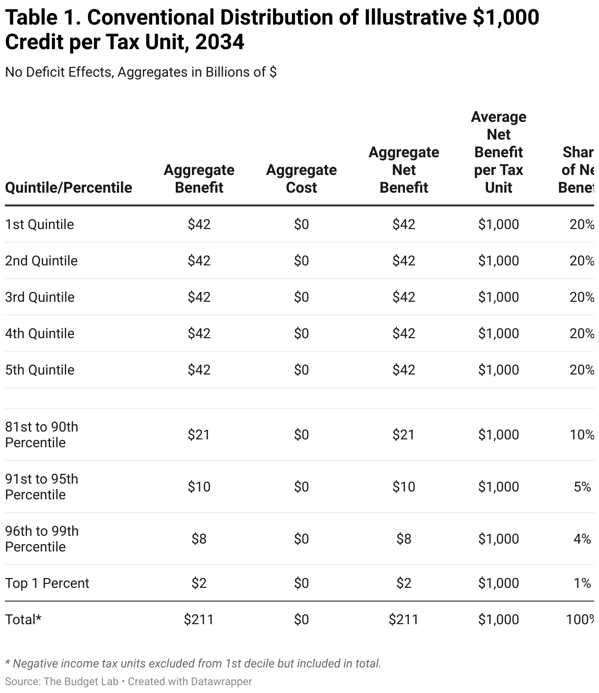
To illustrate the analytical problem, let us consider a simple $1,000 per tax unit refundable tax credit that is not adjusted for inflation. We assume for further illustration that Congress passes this tax credit without any accompanying spending cuts or revenue increases, so the entire cost of the tax credit is deficit-financed.
Without accounting for the means of financing, this policy is straightforward to analyze. Table 1 shows how a conventional distributional analysis approaches the idea looking forward to 2034. Obviously, the average benefit per tax unit is $1,000, and with 211 million projected tax units in 2034 the aggregate benefit would simply be $211 billion. Each percentile would share exactly equally in the benefit, but lower-income groups would see a far larger percent rise in after-tax income as a result of the credit.
A dynamic analysis without accounting for financing would add a few more complexities. It might account for the labor supply response from the credit’s income effects, the implications of investment crowd-out on interest rates and GNP, and, on a long enough horizon, intergenerational effects. But even under a dynamic analysis, it’s unlikely that the labor supply or crowd-out negative effects of this policy would come anywhere close to outweighing the direct benefits of the policy. Putting the merits of the policy itself aside, this approach creates the misleading impression that deficit-financing the policy is strictly superior to offsetting its fiscal impacts with other cuts in spending or increases in revenue.
Options for Distributing Deficits
The Budget Lab considered several questions around distributing deficits.
Distributing Total or Primary Deficit Effects
The Budget Lab distributes total deficits. The most basic question is which measure of deficit effect to distribute in the first place: a policy’s primary (non-interest) effect, or its effect including debt service, i.e. its total deficit effect. One could argue that the total deficit effect overstates the magnitude of the payfor needed to offset a policy’s fiscal effects; that is, paying for a policy with a $1 trillion primary effect over a decade and $200 billion in additional debt service requires policies that together reduce the deficit by $1 trillion, not $1.2 trillion. Moreover, if The Budget Lab were distributing the effects of policy on a Net Present Value (NPV) basis, then including interest payments would be double-counting in that context. However, the goal of this exercise is to capture the consequences of financing choices. To exclude debt service effects would leave out a key financing dynamic. Moreover comparing only primary deficit effects would be imply neutrality between different interest rate regimes, whereas distributing total deficits leads to the intuitive result that a policy enacted under a high interest rate regime would have greater distributional burden in the future than the same policy enacted under low interest rates. Finally, The Budget Lab does not distribute on an NPV basis as the convention employed by other organizations like the Congressional Budget Office and the Joint Committee on Taxation is to show distributional result at discrete future years. Under this approach, including interest costs is not double-counting.
Share of Total Deficit Effect Distributed
The Budget Lab distributes 100% of a policy’s total dynamic deficit effect. A related question is whether a deficit distributional methodology should distribute all, or only a portion, of a policy’s total deficit effect. This question is one of fiscal space, and speaks to the lived experience of the United States in the post-World War II years. Acalin & Ball (2023) calculate that robust economic growth explains between 1/3 and 40% of the fall in debt-to-GDP between 1946 and 1974. While far from explaining the entire drop, it does raise the intriguing methodological choice of allowing for a “growth premium” to “pay” for a portion of a policy.
But in practice, this choice does not make sense for several reasons. First, in periods like the current one in which the baseline debt path is already unsustainable—that is, the net present value of future expected primary surpluses is smaller than the current stock of debt—100% of any marginal increase in debt must by definition be offset in the future with smaller deficits. Even in periods where the starting state is a sustainable fiscal gap, the cost of new policy takes up the fiscal space that another policy or Second, if “fiscal space” is thought of in terms of avoiding unsustainable outcomes—e.g. convex nonlinear increases in debt-to-GDP—the risks run both ways even in periods where growth is expected to exceed interest rates (g > r). g may remain above r, in which case less than 100% of a policy may need to be paid for to avoid some (uncertain) future fiscal inflection point, or r may flip above g, due either to endogenous debt effects on r or entirely exogenous shocks to r and/or g, in which case recovering from a bad outcome might require paying for greater than 100% of the policy. A methodological choice then of distributing 100% of a policy’s cost is a reasonable middle ground. Third, from the perspective of analyzing policy on the margin, the future trajectory of growth and interest rates excluding a policy does not “pay for” the incremental inclusion of that policy. Of course, in a dynamic analysis, it is appropriate to incorporate the marginal economic effects from a policy into the costs and benefits, and these effects would supplement the conventional effects.
Distributional Methods
The Budget Lab distributes deficits by “existing fiscal distribution”. Distributing aggregate deficits requires a prior view about the appropriate method of distribution. There is no objective truth when choosing a distributional assumption for deficits; instead, The Budget Lab considered four different approaches:
- An even across-the-board split between primary spending and revenues;
- Consumption;
- National Income; and,
- “Existing fiscal” distribution (the sum of primary spending and revenue distributions).
The final option merits further explanation. TBL’s “existing fiscal” distribution is constructed by stacking the distributions of mandatory spending (most means-tested benefits as well as social insurance programs like Social Security and Medicare), discretionary spending, and taxes. Taxes, mandatory spending, and discretionary transfers (programs like LIHEAP and WIC) are distributed as-is; other discretionary spending such as defense is distributed on an equal per-tax-unit basis.1 TBL distributes the primary spending and revenue portion of deficit increased based on the spot existing fiscal distribution each year, while it distributes the interest portion based on the cumulative nominal primary spending and revenue effects through each future year.
Each approach has a defensible justification. If the idea is to benchmark the distribution of deficit financing against a neutral alternative, equal spending & revenue cuts are an attractive yardstick. If instead the idea is to benchmark deficit distributions to measures of welfare, then consumption and national income are more appropriate. A consumption distribution also implicitly acts as a VAT payfor benchmark; a national income distribution acts like a tax on factor income. The existing fiscal distribution is essentially the equivalent of an across-the-board equal-proportion primary spending cut (across both mandatory and discretionary spending) and tax hike, with the spending/revenue split depending on the actual division between the two.
Figure 1 shows the 2019 distribution of four metrics capturing these approaches. The orange line shows the Piketty-Saez-Zucman distribution of national income (PSZ), by income decile. The green line shows TBL’s existing fiscal distribution.2 The navy blue line shows the distribution of expenditures from the Consumer Expenditure Survey (CEX), by expenditure decile. The purple line shows PSZ’s distribution of deficits, which is similar to TBL’s “existing fiscal” distribution, with the exception that PSZ 1) constrain the spending-revenue split to be 50-50 rather than as-is/proportional as TBL does; 2) distribute discretionary spending according to national income, rather than flat per-unit as TBL does. Finally, the light blue line shows The Budget Lab’s estimates of the distribution of consumption by income, proxied as the burden of a Value-Added Tax, (cash income less indexed transfers).
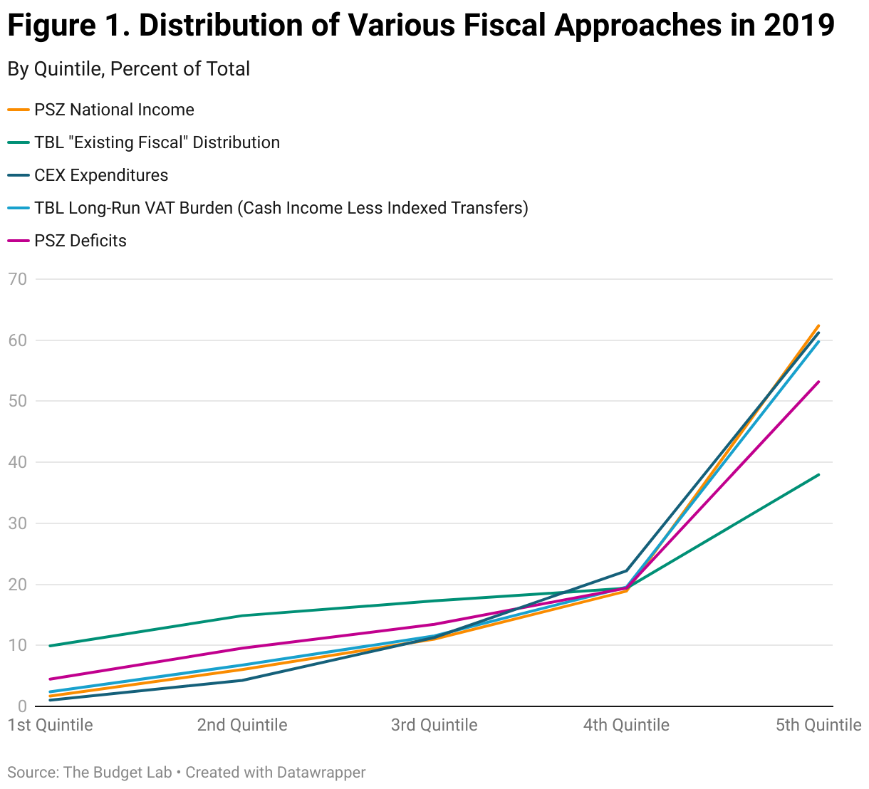
The take-away from Figure 1 is that all five distributions follow similar broad contours, but that the existing fiscal distribution is less progressive than the other three. In particular, note that PSZ national income distributes defense and other “collective consumption expenditure” by pre-tax income rather than on a flat per-tax-unit basis, yielding a more progressives shape than the existing fiscal distribution. The Budget Lab leaned toward the existing fiscal distribution for a number of different reasons. Most prominently, the nexus between the existing fiscal distribution and the goal of the exercise—distributing fiscal deficits—is the strongest. TBL also felt that existing fiscal was the most neutral method, as it implicitly assumes that deficits will be reduced in the future pro rata according to what the government already does on both spending side and revenue side. National income mostly shares that feature as well, but we believe that equal per-tax-unit distribution of defense and related expenditures better accords with the standard convention of distributing spending based on cost rather than on valuation. In contrast, using CEX expenditures or the long-run VAT burden would implicitly assume that deficits will be reduced via consumption taxes that Congress has never adopted.
Illustrative Examples
Flat Per-Tax Unit Credit
Returning to the simple $1,000 per tax unit credit outlined in Table 1: Table 2 below shows how the policy would distribute under The Budget Lab’s chosen existing fiscal distribution methodology in 2034. The benefits still sum up to $211 billion, evenly split across income percentiles. The cost column however now incorporates the financing effects: $211 billion in primary deficits and an additional $74 billion in debt service resulting from 10 years of the policy adding to the debt, for a total of $284 billion to be distributed according to existing fiscal outcomes. Note that Table 2 does not incorporate further dynamic effects, such as long-run crowding out or stimulation of the economy.
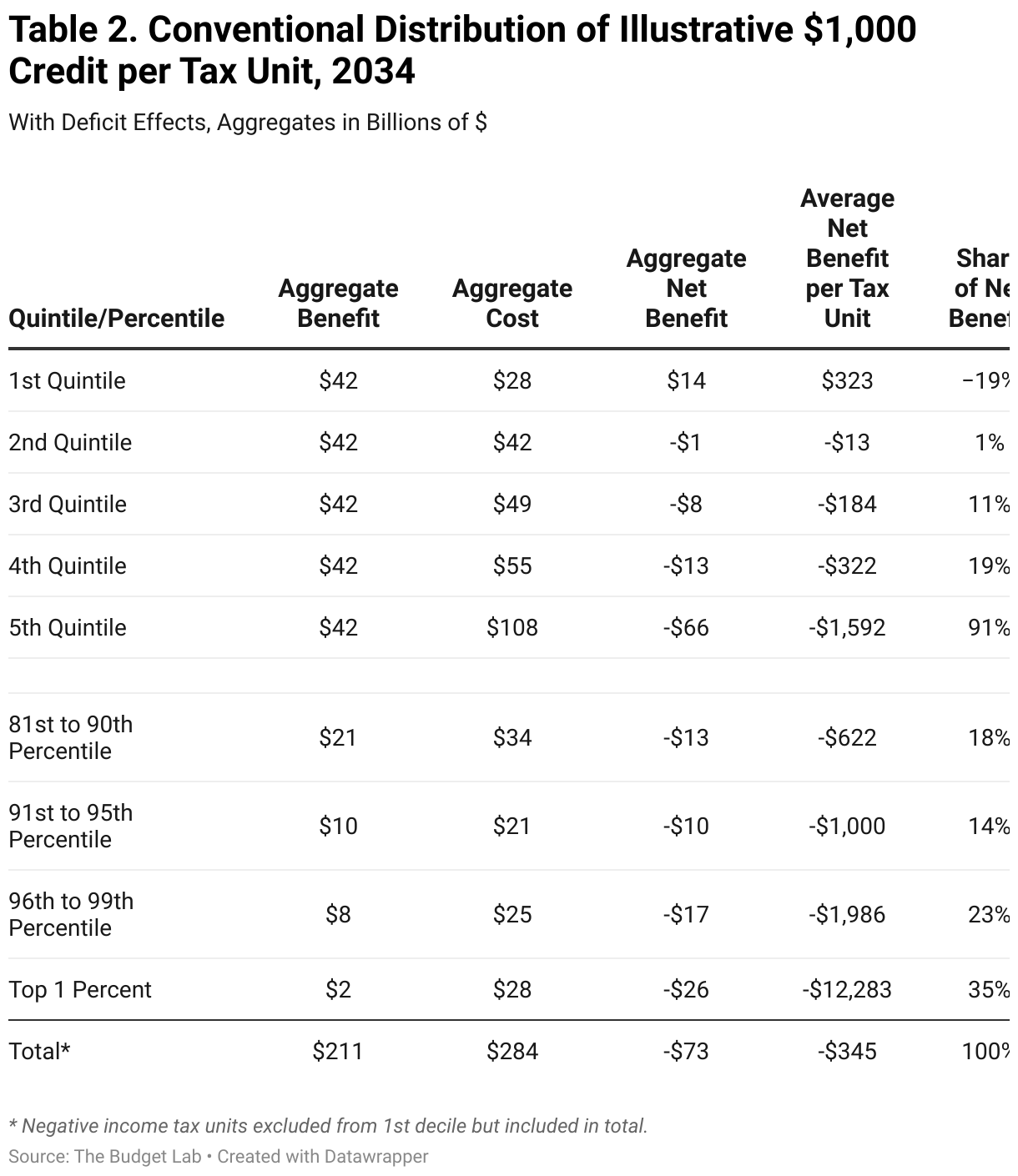
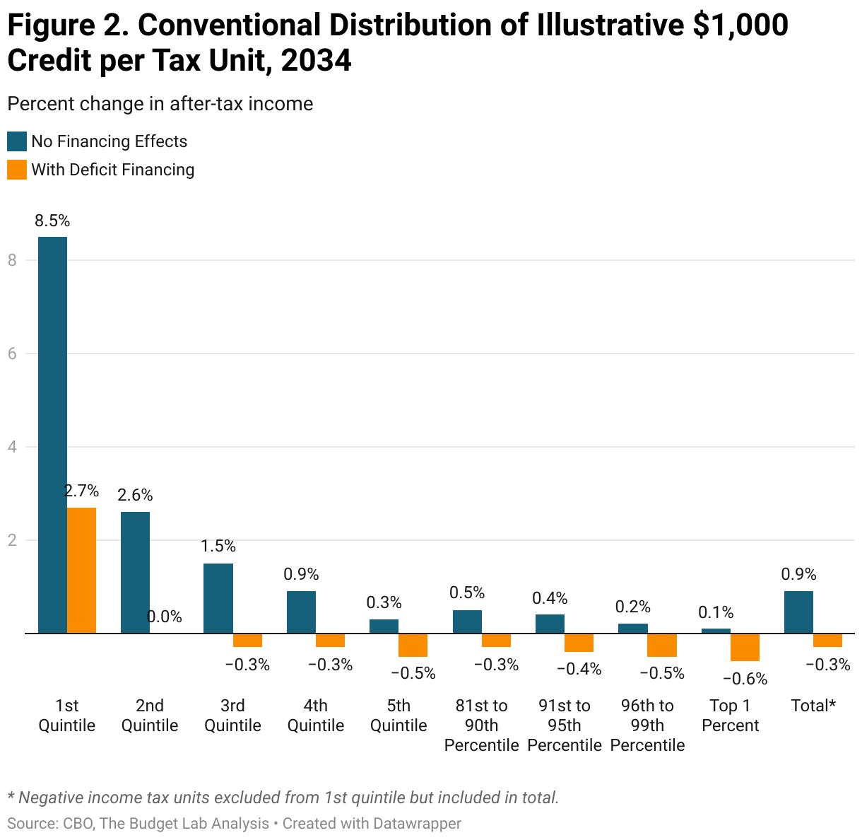
Now, instead of a net benefit, the deficit-financed policy shows a net cost of $73 billion in aggregate (equal to the marginal debt service payments), or $345 per tax unit. But the net benefit varies widely across families: for the first quintile, it is a positive $323 on average, while it is -$12,283 in the top 1%. Again, one way to conceptualize these effects is that this is what the net distribution would look like in 2034 if the total deficit effect of this policy were paid for by proportion, across-the-board spending cuts and revenue increases.
It may seem jarring to go from Table 1, where the benefits were unambiguous and uniform, to Table 2, where suddenly they because negative overall but with a wide variation. It may also not seem intuitive given the flat, straightforward benefit of the underlying policy. But recall that the goal of a deficit distribution is not to capture tangible cash transactions, but rather to incorporate financing costs at any given future point in time since, under the government budget constraint, all debt will have to be paid off eventually. So in Table 2, it is not that the top 1% will literally be worse off by $12,283 per tax unit in 2034, rather it is that financing costs accumulate over time and weigh on national income, and at the discrete moment of 2034, closing the fiscal gap opened up by deficit-financing the policy with proportional adjustments suggests the top 1% would shoulder $12,283 in costs per household on average, much more than the $1,000 direct benefit each would receive from this policy. This also illustrates the temporal trade-offs for policymakers: the longer they wait to “pay off” a policy, the larger the aggregate burden and the more material the distributional effects.
Can aggregate net benefits ever be positive under our approach, or are they constrained to always be negative and equal to the debt service cost? A conventional analysis will always be equal to the aggregate net financing cost under the Lab’s methodology. But this is where dynamic analysis can add further value. A high-multiplier fiscal policy—say, a temporary one passed in a macroeconomic environment of high resource underutilization, low supply chain constraints, low interest rates, and an accommodative Federal Reserve—could easily bring a net benefit in the short-term, before marginal debt effects have time to accumulate and drive up financing costs. Similarly, a policy with a marginal-value of public funds above around 6 (reflecting how much value a policy has to drive before it pays for itself in taxes given current taxes as percent of GDP in the United States) could also result in a dynamic analysis that shows aggregate positive net benefits. The Budget Lab’s methodology would also distribute these positive short-run dynamic effects according to existing fiscal effects.
Note too that TBL’s distributional approach is symmetric: a policy that reduces the deficit will, over time, have less of an aggregate cost under our financing approach, and less of a cost for any given distributional cohort, than a conventional analysis that does not account for financing.
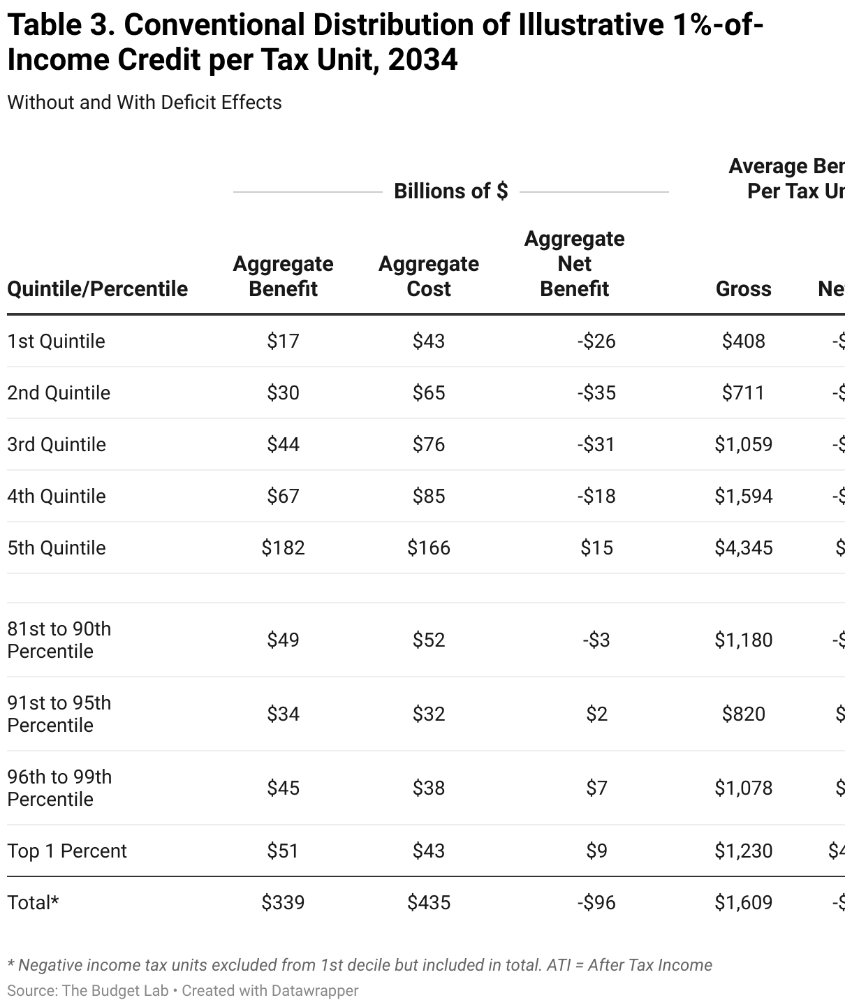
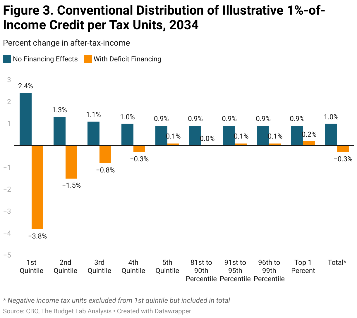
Proportional 1%-of-Income Tax Credit
What about a proportional tax cut? The table below shows the distribution in 2034 of an illustrative refundable tax credit equal to 1% of before-tax income. As you can see, judged against after-tax income, the gross benefit distribution of this policy is mildly progressive: the bottom quintile sees an increase of 2.4% to their after-tax income, while the top 1% see a 0.9% increase. The net benefit distribution incorporating financing costs is much different, showing a regressive policy, with the bottom quintile bearing a 3.8% loss in income while the top 1% still see a net 0.2% increase.
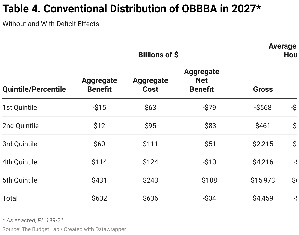
OBBBA
Finally, what about more complex policies? Here, we show how TBL’s recent distribution of OBBBA changes under our deficit distribution framework. Under a gross benefits approach, the package is regressive, with a 3% fall in bottom quintile income versus a 6% rise in top quintile income, a swing of about 9 percentage points. The package is even more steeply regressive when incorporating deficit costs however: the net benefit swings from a 14%-of-income burden at the bottom to a 3% benefit at the top, a swing of roughly 17 percentage points.
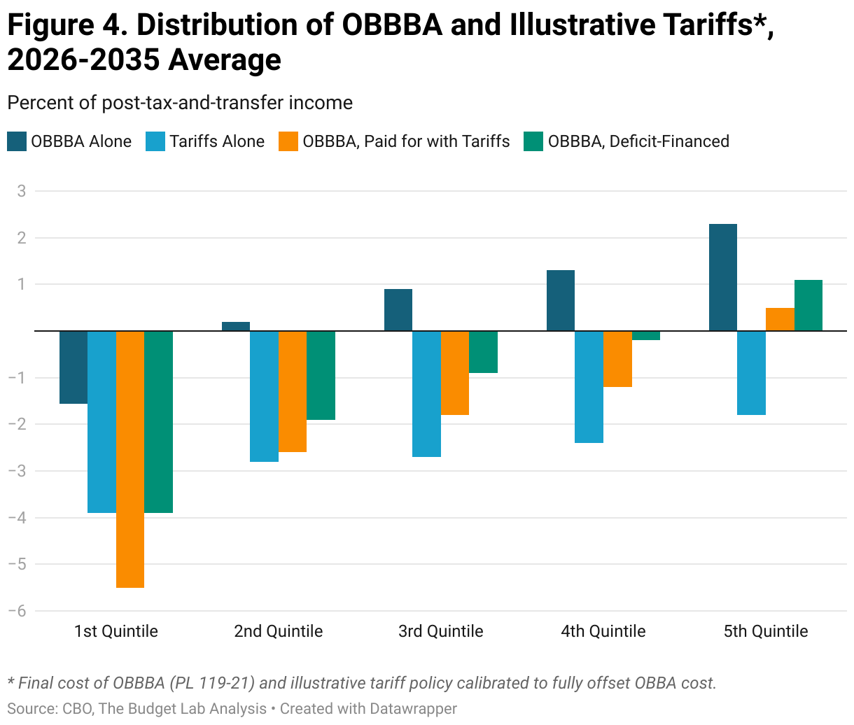
The final OBBBA as enacted was scored by CBO as raising the primary deficit by $3.4 trillion over 2025-2034 against current law; we estimate CBO would score OBBBA as costing $3.7 trillion expanding the window one-year further to 2025-2035. Meanwhile, CBO also projects that tariff policy as of mid-August would raise $3.3 trillion over 2025-2035. On an apples-to-apples basis, then, current tariff policy would almost but not quite cover the cost of OBBBA over the next decade should both remain in place and unchanged.
An instructive comparison, then, is how the distribution of OBBBA, paid for with tariffs sufficient to raise $3.7 trillion through 20353, compares to a deficit-financed OBBBA under our methodology. The figure below compares our distributional results. Deficit-financed OBBBA is regressive but less so than tariff-financed OBBBA, with the biggest differences arising in the first and fourth quintile. This suggests that proportionally raising taxes & cutting spending has a distributional impact less regressive than TBL’s approach to distributing tariffs.
Conclusion
The Budget Lab's methodology for distributing the costs of deficit-financed policies in distributional tax analysis addresses key challenges and makes informed choices on several critical decisions. The Lab’s approach offers a comprehensive framework for evaluating the short- and long-term distributional impacts of fiscal policies with financing considerations incorporated. It provides a more holistic view of the true costs associated with deficit financing, addressing limitations in current analyses that often overlook long-term implications. As fiscal challenges continue to evolve, such comprehensive analytical frameworks will be crucial in shaping effective and equitable economic policies.
Footnotes
- While higher-income families may have a higher willingness-to-pay for certain discretionary government services, TBL decided on a flat per-unit distribution of non-transfer discretionary spending as it better approximates how services would be distributed under market pricing and government transfer. E.g. imagine there were a “market” for national defense, selling at a single price that is, in a competitive market, roughly at cost. The U.S. government corners this market and distribute national defense to all Americans (and prevented households from buying more). The final distribution of national defense would approximate a flat per-unit distribution based on the “market” price. There are obviously some discretionary services that upper-income families utilize more than lower-income ones (e.g. judicial contract enforcement), but there are others they utilize less (e.g. certain educational grants), so flat per-unit is still a reasonable compromise.
- Data for the 2019 existing fiscal distribution comes from CBO’s Distribution of Household Income. CBO’s distribution is by household in this report; the differences between distribution by household, tax unit, and per adult are not substantial.
- Under TBL’s estimation, it would take a roughly-7 percentage point increase in the average effective tariff rate, from 17.4% as of September 4 to 24.6%, to raise the total amount of revenues from new 2025 tariffs to $3.7 trillion through 2035.