
“Buy-Borrow-Die": Options for Reforming the Tax Treatment of Borrowing Against Appreciated Assets
Key Takeaways
-
Current tax law favors borrowing over selling appreciated assets. We explore three targeted reform options aimed at neutralizing this tax preference: treating borrowing as a taxable event (“deemed realization tax”), requiring prepayment of capital gains tax at time of borrowing (“withholding tax”), and a flat tax on certain loans (“excise tax”).
-
Estimated ten-year revenue impacts range from $102 billion to $147 billion, with wealthy taxpayers generally seeing the largest tax hikes.
-
The deemed realization tax and the withholding tax would eliminate the tax preference for borrowing for most taxpayers. The excise tax, on the other hand, would leave the tax preference in place for some while also newly taxing others who are borrowing for legitimate non-tax reasons.
Introduction
Designing a potential extension of the Tax Cuts and Jobs Act (TCJA) is the central tax policy question facing Congress in 2025. Because a straightforward extension of the TCJA would come with a fiscal cost of more than $4 trillion over ten years, lawmakers and policy experts have expressed interest in incorporating additional revenue-raising provisions into an extension package—often with a focus on areas where fundamental reform would be beneficial.
One such area is the so-called "buy-borrow-die" strategy, a tax planning technique which allows wealthy Americans to pay low tax rates on consumed income, creates horizontal inequities, and distorts portfolio allocation decisions. Buy-borrow-die has attracted growing attention from economists, legal scholars, and politicians seeking ways to reform how capital gains are taxed in the US.
In this report, we:
- Explain how the existing tax code gives rise to the buy-borrow-die strategy
- Explore three reform options and highlight policy design tradeoffs
- Estimate the revenue potential and distributional impact of each reform
- Measure the tax advantage for borrowing under current law and each reform
Background
Capital gains are generally tax-advantaged relative to other types of investment income. In addition to facing lower statutory rates, capital gains enjoy two other advantages:
- Taxation upon realization. The US tax code generally requires that income be realized in order to be taxable, a principle which confers a unique tax advantage to capital gains. Gains are taxed upon realization (when an appreciated asset is exchanged for cash) rather than upon accrual (when the asset appreciates). As such, taxpayers whose income takes the form of assets rising in value (versus, say, income in the form of wages or interest) have significant flexibility over when to pay taxes. They can strategically choose to realize gains in years when they face lower tax rates, and more broadly, deferral of tax liability reduces its present value via the time value of money.
- Stepped-up basis. When assets are inherited, their cost basis is "stepped up" to fair market value at the time of death. This eliminates any accumulated would-be capital gains tax liability on appreciation that occurred during the deceased's lifetime, allowing all lifetime income taking the form of unrealized appreciation to completely escape taxation.
Together, these features create a simple tax strategy for those looking to maximize the amount of wealth passed onto their children: hold onto low-basis assets until death and finance any consumption needs through other income sources.
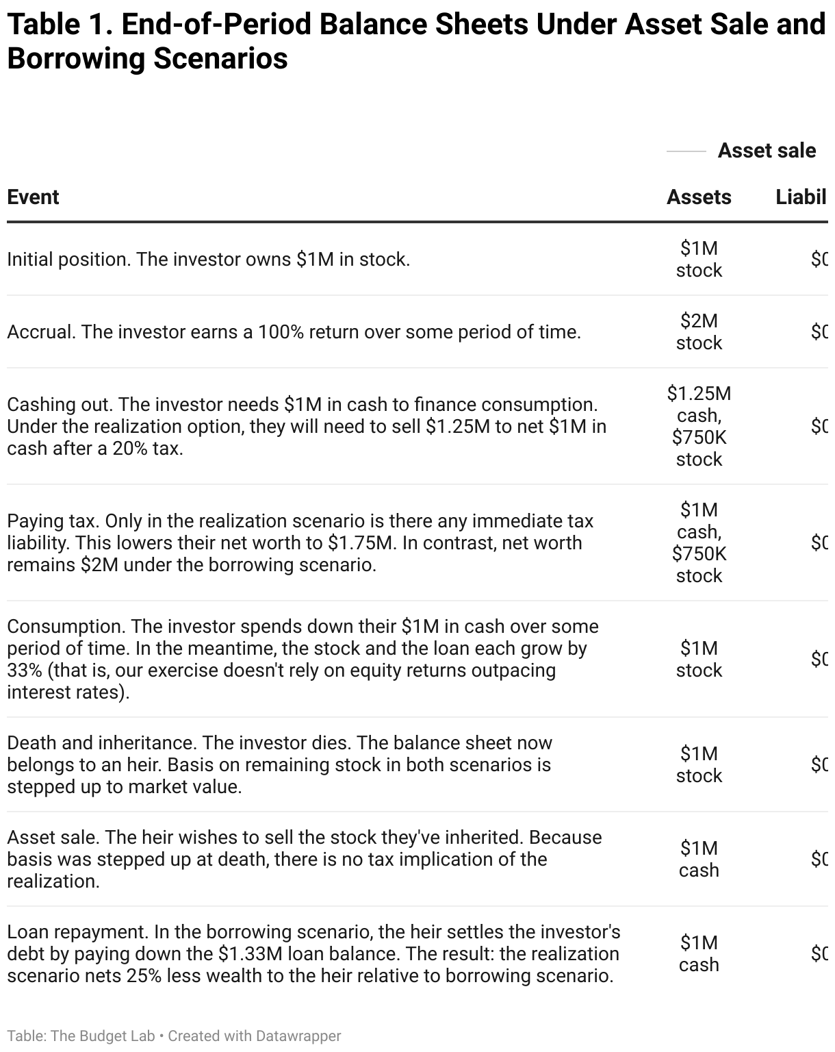
One such income source is borrowing against the value of appreciated assets. Loan proceeds are traditionally nontaxable, as they represent a temporary transfer of cash that will be repaid, not income per se. But in the case of someone borrowing against appreciated assets, loan proceeds function identically to cash from an asset sale—except without the associated tax liability. This is the “buy-borrow-die" strategy, which results in appreciation escaping tax entirely. An example helps illustrate how this strategy works:
This strategy creates several issues for efficient and fair taxation:
- Horizontal inequity. Current law treatment of borrowing violates the principle of horizontal equity—the idea that taxpayers with similar total incomes should face similar tax burdens. Current law favors those who finance consumption through borrowing rather than selling assets, and it favors investing in assets that generate capital gains over those that pay dividends or interest. This kind of horizontal inequity encourages inefficient tax avoidance and is associated with notions of unfairness.
- Vertical inequity. The ability to execute a buy-borrow-die strategy is disproportionately available to wealthy households. These taxpayers are more likely to earn a substantial fraction of their economic income through capital gains—a pattern that is especially true among multi-billionaire founder-executives who hold low-basis, liquid shares in the world’s most valuable companies. Wealthy households also have better access to complex financial products and tax planning services.
- Lock-in effect and economic inefficiency. The tax advantage for borrowing over realization creates a “lock-in” effect in which investors face strong incentives to hold onto appreciated assets even when they would otherwise prefer to diversify or reallocate their portfolios. All else equal, a concern for tax efficiency over allocative efficiency distorts price signals in financial markets.
Underlying buy-borrow-die as a viable strategy is the tax preference for consuming out of loan proceeds rather than asset sales. How large is this preference? To answer this question, we develop a simple mathematical model described in the Appendix. Under plausible assumptions about cost basis, interest rates, and more, we estimate that the current-law tax rate on borrowing is about 12 percentage points lower than the tax rate on selling. An expanded discussion of the tax advantage is the subject of a section below.
Finally, it’s worth noting that while buy-borrow-die is a well-documented tax planning strategy with several high-profile cases, borrowing against assets appears to be a relatively minor source of cash income for wealthy Americans in the aggregate. Liscow and Fox (2025) find that borrowing (of any kind) represents only 1% of the income of the top 0.1% by net worth. This means that reforms designed to include loan proceeds in taxable income will be somewhat limited in their revenue potential compared with more fundamental reforms of capital income taxation. Still, from a first-principles perspective, policy changes aimed at limiting buy-borrow-die are a natural place for reform in the current tax code.
Options for Reform
As shown above, the fundamental driver of buy-borrow-die is the ability to defer gains in the expectation of stepped-up basis at death. There is a wide array of proposed reforms that would tackle these issues head on—reforms which, as a side effect, would shut down buy-borrow-die as a viable strategy.
In this report, however, we focus on three targeted approaches for limiting buy-borrow-die by focusing on the “borrow” portion. These options are not designed to disallow deferral or erasure of gains at death entirely. Rather, the goal is to disallow deferral that is motivated by borrowing-related tax arbitrage.
To help make our proposed reforms options concrete, we show how three representative taxpayers would be affected by each proposal in the Appendix.
Option (1): Deemed Realization for Borrowing
This option, based on a proposal by Liscow and Fox (2024), would treat loan proceeds as a “deemed realization” of unrealized capital gains. That is, borrowing would be treated as a realization event. After tax is paid, the basis of the affected assets would reset to fair market value, preventing double taxation if the assets are later sold.
Taxpayers would not get to choose which specific assets are used for deemed realization. Rather, cost basis would be determined on a first-in-first-out basis. For example, if a taxpayer borrows $10M and their oldest $10M in assets have a basis of $1M, then the taxpayer is treated as having realized $9M in gains. If instead they borrowed $10M but their oldest $10M in assets have a basis of $10M, no tax is owed. In this way, the tax is conditioned on having unrealized capital gains (rather than simply being a tax on loan proceeds) and thus represents an integration with the existing income tax system.
Remaining design details for this option differ slightly from those of the Liscow-Fox proposal:
- Tests for applicability. Liscow and Fox propose three tests to determine whether a taxpayer is subject to the borrowing tax: a $100M net worth threshold requirement, a lifetime borrowing exemption of $1M, and an annual exemption of $200,000. In contrast, this reform option would apply to all taxpayers and include an annual inflation-indexed exemption of $250,000 (or $500,000 for joint returns). That is, households are allowed to borrow up to $250,000 per person per year before facing any tax.
- Covered borrowing. Liscow and Fox would include new debt of any kind in the tax base, regardless of whether that debt was secured by pledged assets, as is often the case in buy-borrow-die arrangements. The idea is that if the tax applied only to securities-based lines of credit, affected households could avoid the tax by shifting their collateralized borrowing into other types of loans like recourse borrowing or forms of implicit backing. Option (1) would include all borrowing except the following: primary residence mortgages, student loans, auto loans, and credit card debt. This definition creates a tax base that includes securities-based loans, unsecured non-card lines of credit, margin loans, non-primary residential debt, and more. While exempting certain categories may open the door for abuse in some cases, these forms of debt would be difficult to game and their exclusion is required for progressivity (given that this option does not include a net worth test for applicability).
- Tax rate. Liscow and Fox’s proposal is designed to be consistent with the FY 2024 President’s Budget, which called for a top rate on capital gains of more than 45 percent. Instead, this option would tax borrowing at the current-law top combined rate of 23.8 percent. This rate is invariant with respect to taxpayer income; therefore, some taxpayers would face a lower tax rate on asset sales.
- Retroactivity. While Option (1) would tax new borrowing only, Liscow and Fox propose including existing loans in the tax base. This design choice would function as a one-off transition tax, which would raise additional revenue without distorting economic decision-making but might raise questions of fairness.
Option (2): Withholding Tax on Borrowing
This option would apply a simple flat-rate “withholding” tax on loan proceeds, with the withheld amount creditable against future capital gains tax liability. Under the proposed 10% withholding rate, a $10 million loan would trigger an immediate $1 million tax payment regardless of the taxpayer's basis in their assets.
The withheld amount functions as a pre-payment of future capital gains tax. If taxpayers realize capital gains later in life, they can credit their withholding tax payments against the capital gains tax liability. At death, any excess withholding above implied capital gains liability would be refunded, while any shortfall would be collected before basis step-up applies.
This option can be understood as a variant of Option (1): both proposals impose deemed realization for borrowing against appreciated assets, but they collect this tax at different times. Option (1) determines and collects liability at the time of borrowing; Option (2) collects some tax at the time of borrowing then reconciles this prepayment with actual liability when assets are sold or at death. This difference shifts the administrative burden of valuing assets and reporting basis from the time of borrowing to the time of realization or death. Whether Option (1) leads to lower tax burdens than Option (2) depends on taxpayer-specific details like cost basis and investment returns; see the section below on estimated tax advantages for further discussion.
The remaining details would be identical to those of Option (1): a $250,000 per-person per-year exemption and a definition of taxable borrowing that excludes certain mortgages and installment loans.
Option (3): Annual Excise Tax on Loan Balances
This reform, based in part on a Bipartisan Policy Center proposal, would impose a 0.5% annual tax on the outstanding balance of covered loans.1 In contrast with the prior two reform options, which would apply to net new flows of borrowing, this option would apply to the stock of debt. For example, a $10 million loan balance would incur an annual liability of $50,000.
This option would cover the same categories of lending as Options (1) and (2). But unlike those reforms, this one would not include an exemption before tax applies. The tax would be administered at the lender level, meaning that the institution that originates a taxable loan, not the borrower, would be legally required to remit the tax.
Rather than attempt to measure and tax underlying appreciation, as with Options (1) and (2), this proposal operates as a direct increase in borrowing costs for these tax-advantaged financing arrangements. While this approach is less precisely targeted than the others and may discourage borrowing for reasons unrelated to tax avoidance, it benefits from the administrative simplicity—taxpayers would not have to report and update basis when they borrow, and its firm-level structure means that there are fewer taxpayers burdened with compliance costs.
Tradeoffs in Policy Design
The design choices embedded in these reform options reflect inherent tensions in reforming the tax treatment of borrowing. There are several important dimensions along which policymakers must trade off potential goals:
- Wealth and income tests: progressivity vs administration. Given that buy-borrow-die is a tax strategy used generally by the wealthiest Americans, one design question is whether to condition on wealth directly. This kind of net worth test would definitionally achieve any goals for progressivity. However, a wealth test would require regular valuation of complex asset portfolios, potentially straining IRS resources and creating opportunities for avoidance through sophisticated ownership structures. Another alternative for progressivity is an income-based test. This would require no additional reporting, but income is not perfectly correlated with wealth and may fail to identify high-net worth households with low taxable income—a defining characteristic of those who are engaging in buy-borrow-die. The absence of wealth or income tests, as in Options (1) and (2), simplifies administration at the cost of affecting a broader range of taxpayers. This approach relies more heavily on exemption levels to achieve progressive effects.
- Exemption levels: progressivity vs avoidance. A high annual borrowing exemption reduces the fraction of taxpayers subject to tax, creating a system that only burdens those with high amounts of borrowing—households who are, with some rare exceptions, wealthy. But the higher the annual exemption, the more that taxpayers can avoid by spreading their borrowing out across multiple years. An alternative to an annual exemption is a lifetime exemption, as in the case of the estate and gift tax. This would eliminate the possibility for avoidance via debt smoothing but come at the cost of administrative complexity, as taxpayers and the IRS would need to track cumulative lifetime borrowing over time.
- Tax base: targeting vs avoidance. Exactly which forms of borrowing should be covered by the tax is a question where comprehensiveness is balanced against avoidance opportunities. On one extreme is the case where only securities-based lines of credit are subject to the tax, which would target tax-motivated borrowing with precision but create opportunities for shifting into other kinds of debt products. The other extreme is a tax that applies to all forms of debt, which would prevent substitution between loan types but have the potential to affect routine household borrowing. This tradeoff can in part be mitigated by the presence of other design features, for example a wealth test (in which case a comprehensive base prevents borrowing without the risk of taxing normal household finance). Options (1) and (2) take a middle-ground approach by excluding specific categories of consumer debt—those that are common to middle-income families and are unlikely to be tools of sophisticated tax planning—while maintaining broad coverage of other borrowing.
- Integration with income taxes: efficiency vs administration. The purpose of integrating a new borrowing tax into the existing income tax system is to create tax neutrality between borrowing and selling, which in turn reduces tax-driven distortions in household financial decision-making. Full integration through deemed realization, as in Option (1), creates neutrality between borrowing and selling appreciated assets—but at the cost of new administrative burdens, since it requires valuing assets, imputing realizations, and updating basis at the time of borrowing. Option (2) is a form of partial integration, since the withholding tax is calculated without regard to basis at the time of borrowing. Relative to Option (1), this reduces initial compliance costs, shifting them to time of sale or death—events where the IRS already has some administrative infrastructure in place. The least integrated approach described above, a tax on the stock of loans remitted by the lender, offers administrative simplicity: the burden is shifted from households to large institutions, and the calculation itself is simple. But this advantage is traded off against the goal of achieving tax neutrality for all taxpayers. While the tax rate can be calibrated to achieve tax neutrality on average, differences across taxpayer circumstances means that there will still be a distribution of tax preferences for borrowing at the household level.
Estimated Budgetary Effects
This section presents conventional revenue estimates for each of the three reform options. These estimates, which reflect the effects of behavioral feedback, come from a microsimulation model based on the Survey of Consumer Finances (SCF). Additional modeling details can be found in the Appendix.
Table 2 shows estimated annual budget effects over the ten-year budget window and totals for the following two decades. We estimate that within the budget window, reform Options (1), (2) and (3) raise $102, $147, and $130 billion respectively.
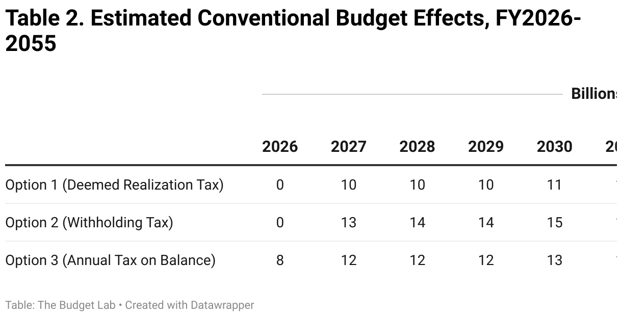
While Options (1) and (2) are similar in design, the latter would raise more revenue due to timing differences. In Option (1), if a borrower secures a loan but has no unrealized capital gains, they owe no taxes. However, under Option (2), a borrower in the same situation owes 10% on the value of the new debt. While this payment will be credited against tax at time of eventual sale or death, this reconciliation happens in a future year, meaning that the inflows of revenue are larger for Option (2) over any fixed window of time.
These estimates account for two kinds of tax avoidance strategies:
- Intertemporal shifting of borrowing. Taxpayers may re-time their borrowing such that they "use up” the annual tax-free exemption. For example, a taxpayer who under current law would borrow $1.5 million in one year may instead break that loan into chunks, borrowing $500,000 each year for three years and avoiding tax entirely. We assume that households can shift non-housing borrowing of up to 100% of the exemption amount into other years, effectively doubling the exemption that binds. We estimate that this strategy’s effect reduces the number of 2026 taxpayers from 318,000 to 295,000 for Option (1) and from 375,000 to 352,000 for Option (2).
- Closely held businesses as tax shelters. Current law already generates an incentive for owners of closely held businesses to characterize personal consumption expenditures as intermediate business inputs to generate tax deductions. All three reform options strengthen this incentive: debt on the firm’s balance sheet used to finance legitimate business expenditures would be nontaxable, but that same debt would be subject to tax if held on the owner’s personal balance sheet instead. While this kind of abuse would be prohibited explicitly, the IRS would likely have some trouble with enforcement as is the case with the current-law incentive for "consuming out of the firm”. Using an elasticity of business consumption tax sheltering derived from Leite (2024), we estimate that this tax planning strategy would reduce revenue raised between about 2% and 6% depending on the scenario.
Estimated Distributional Effects
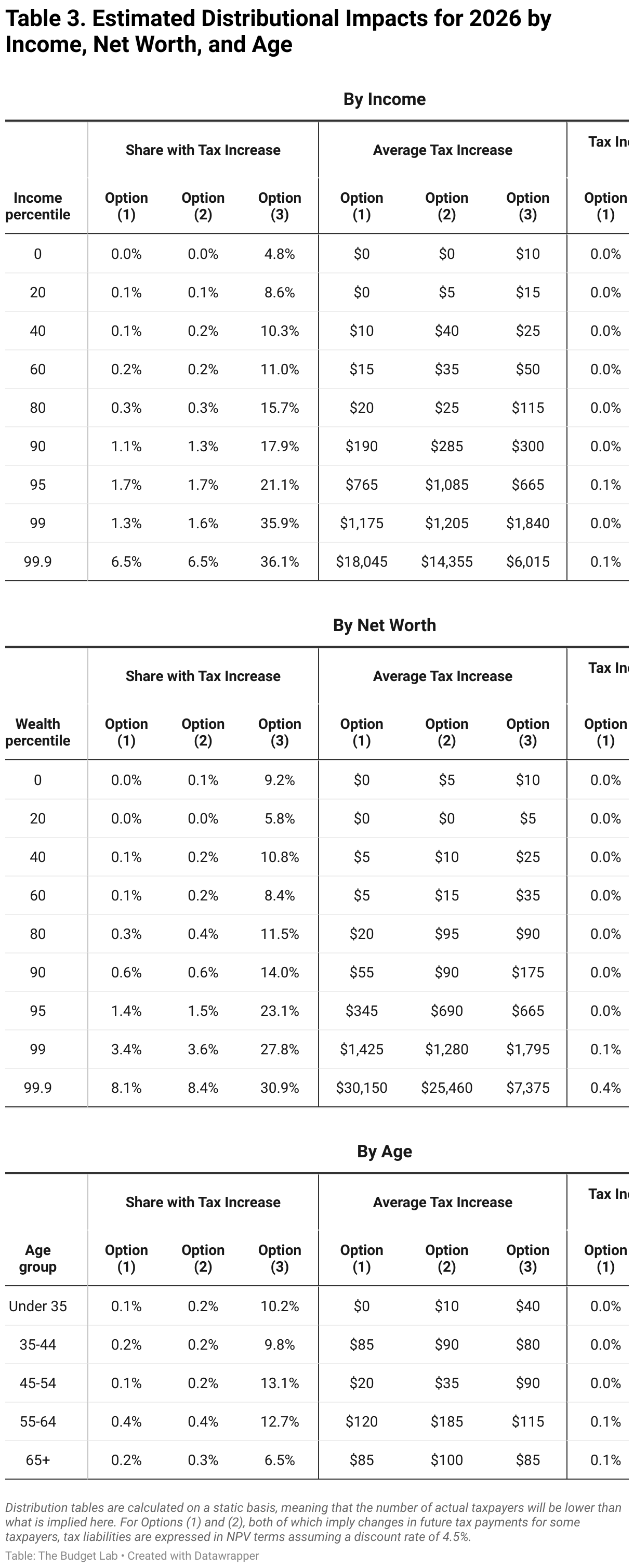
Borrowing and unrealized gains vary by socioeconomic group. Because each reform approaches the taxation of these activities differently, impacts will vary across the population. Table 6 presents a breakdown of estimated effects by income, net worth, and age.
These results underscore several points about buy-borrow-die and policy design:
- Taxing all debt casts a wider net than taxing new debt only. Options (1) and (2) represent more targeted tax increases, affecting less than 1 of the bottom 90% of taxpayers by income. This is because they tax flows of borrowing and are at least somewhat conditioned on having unrealized capital gains. In contrast, Option (3) taxes the stock of debt and is applied regardless of a taxpayer’s unrealized gains. For that reason, a much broader share of households would see a tax increase under Option (3)—many of whom are borrowing for reasons unrelated to tax avoidance.
- Timing of tax payments matters. Options (1) and (2) can be thought of as the same essential policy—a tax on borrowing up to the amount of unrealized gains—but with timing differences. For taxpayers with a high cost basis, Option (2)’s 10% withholding tax on borrowing imposes a larger burden than Option (1) does, essentially collecting a tax on unrealized gains that don’t (yet) exist. Eventually, the taxpayer is credited with any overpayment when they sell or die, leading to the same nominal treatment as in Option (1). But this “interest-free loan” to the government is costly in net present value terms. For that reason, groups with a higher average cost basis see higher taxes under Option (2) than Option (1); the opposite is true for groups with a lower average cost basis, like the top 0.1% by income.
- Taxable borrowing is most common in the decade before retirement. Those in the 55-64 group are about twice as likely as seniors to see a tax increase under all three reform options. While borrowing is most common among younger households within the top wealth group (Liscow and Fox 2025), lifecycle effects mean that younger households tend to be poorer and therefore would be relatively less impacted by these reforms.
Estimated Effects on the Tax Advantage of Borrowing
Beyond raising revenue progressively, these reforms aim to address a fundamental distortion in the tax code: the implicit preference for borrowing over realizing capital gains. By assessing a tax on borrowing against appreciated assets, each reform would reduce the current-law tax advantage for financing consumption through debt rather than asset sales. In this section, we measure the size of these changes in tax treatment.
To do so, we develop a simple model that calculates effective tax rates (ETRs) under different financing choices. It asks the following question: given unrealized gains, expected financial conditions, and a set of tax rules, how much more wealth can an investor expect to pass on to their children by borrowing rather than selling assets? A full description with equations can be found in the Appendix.
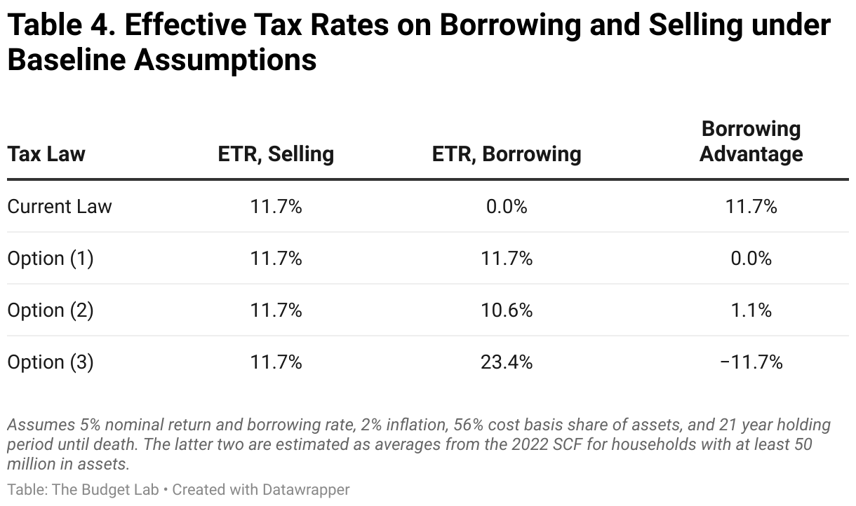
Table 7 shows our baseline estimates of the borrowing tax advantage. We find that, for the average wealthy taxpayer who expects to hold gains until death, financing another dollar of consumption by borrowing rather than selling enjoys an approximately 12pp tax rate advantage under current law. Option (1) would result in tax parity between borrowing and selling, Option (2) would generate approximate parity, and Option (3) would flip the preference towards selling.
These calculations, however, are sensitive to taxpayer characteristics. The effect of each reform option on the tax advantage for borrowing depends on cost basis, expected returns, number of years until death, and more. Below are several important takeaways about these differential impacts:
- Option (1) reduces variance in tax treatment across taxpayers. Option (1) results in tax parity between borrowing and selling for most taxpayer situations. This is because it is integrated with the existing income tax: taxable borrowing is limited to unrealized gains, and it collects tax in the year of borrowing. Simply put, this treats borrowing and selling identically under tax law.
- Option (2) favors those with low cost basis. One way to understand the 10% withholding tax is that it’s equivalent to Option (1)’s 23.8% deemed realization tax when cost basis is 1 - 10% / 23.8% = 58% of asset value in the year of borrowing. For those with a cost basis share less than 58%—that is, those with larger unrealized capital gains—Option (2) is preferable to Option (1) because the taxpayer gets to defer a greater fraction of tax on gains. The opposite is true for those with higher cost basis. All else equal, a basis share of 10% creates a 6pp tax advantage for borrowing under Option (2); a basis share of 90% creates a 13pp advantage for selling. This latter case is less of a concern, since those with a high cost basis—that is, low unrealized gains—are definitionally not likely be borrowing for tax-motivated reasons.
- Option (3) also favors those with low cost basis. Among all three proposals, Option (3) is the least targeted towards buy-borrow-die because it is not tied to unrealized gains in any way. In other words, Option (3) would tax many households who are borrowing for reasons unrelated to tax arbitrage. For that reason, it would generate a borrowing advantage of 4pp for those with 10% cost basis share (larger unrealized gains) and a selling advantage of 21pp for those with 90% cost basis share (smaller unrealized gains).
- Option (3) heavily taxes long-duration loans. Because Option (3) is an annual tax on the stock of debt rather a tax on new debt, its burden falls more heavily on those who plan to borrow for longer amounts of time. All else equal, shortening the assumed duration of borrowing from 21 years to 5 years creates a 7pp advantage for borrowing. But for a 50-year loan, the ETR on borrowing is more than 50pp higher than that of selling.
- Borrowing is still generally tax-favored when returns exceed borrowing costs. Our exercise assumes that the tax-conscious investor is investing in safe assets—a pure tax arbitrage scenario. But what if they borrow to invest in riskier equity assets with a higher expected return? In this scenario, borrowing is still generally taxed advantaged even under the reform options. This is because each option leaves stepped-up basis at death intact, excluding gains that were constructively realized through borrowing. So when taxpayers can borrow at lower rates and invest the proceeds at higher rates, the additional net income margin will go untaxed at death, creating an advantage for borrowing over selling.
Appendix
Illustrative Examples
To help make our proposed reforms options concrete, we show how three representative taxpayers would be affected by each proposal.
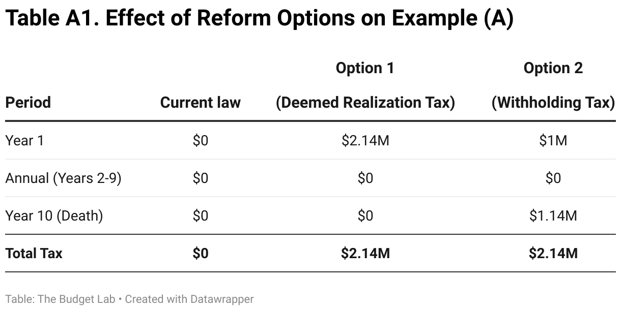
Example (A): Large Loan, Low Basis
A married wealthy taxpayer borrows $10.5 million. Their oldest assets worth $10 million have a cost basis of $1 million, meaning they have an unrealized gain of $9 million. After borrowing, they live for an additional ten years and do not sell any assets during this period. For simplicity, we assume that the loan balance does not grow over time.
After accounting for the $500,000 exemption, Options (1) and (2) generate $10.5 million - $500,000 = $10 million in covered borrowing. Option (1) limits taxable borrowing to the $9 million unrealized gain, leading to $2.14 million in tax based on the 23.8% rate. Option (2) collects $10 million x 10% = $1 million upfront but requires an additional $1.14 million payment at death to match the full tax on gains—the same nominal liability as Option (1), but lower in present value terms. Option (3) simply charges a flat 0.5% tax on the $10.5 million annually, leading to annual payments of $52,500 and $525,000 over 10 years.
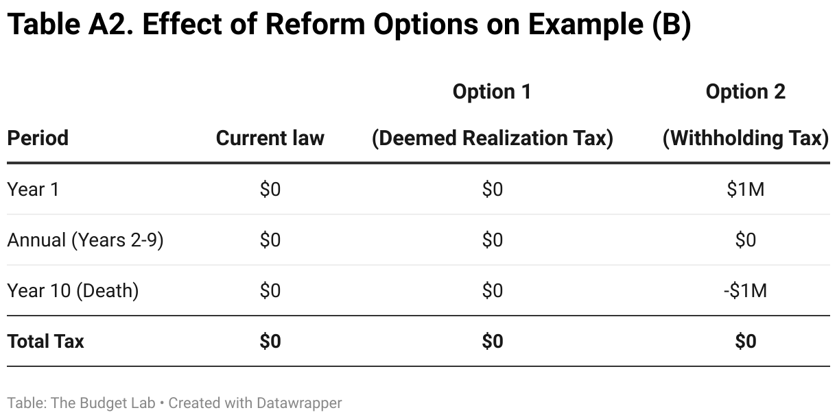
Example (B): Large Loan, High Basis
This example is identical to Example (A) except the cost basis is $10 million, meaning they have no unrealized gains on these assets.
Option (1) triggers no tax because there are no gains to constructively realize. Option (2) still collects $1 million upfront but refunds it fully at death due to lack of gains. But Option (3), which is not tied to the circumstances of unrealized gains, charges the same $52,500 annual tax as that of Example (A).
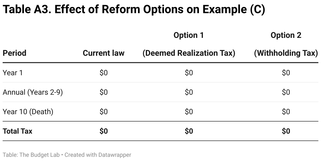
Example (C): Smaller Loan
In this example, a married couple borrows $500,000 to finance the purchase of a vacation home. Their oldest $500,000 in assets is zero-basis equity in a closely held business. As above, they live for an additional ten years and do not sell any assets during this period.
Options (1) and (2) impose no tax because the annual exemption is $500,000. Option (3), however, taxes the balance at a rate of 0.5%, totaling $25,000.
Revenue Estimation Methodology
This section details our approach to estimating the revenue effects of the proposed reforms. The code for our analysis, which contains precise details for all calculations described here, can be found here on the TBL Github page.
Our analysis begins with several data sources:
- Survey of Consumer Finances (SCF). This cross-sectional survey microdata serves as our primary source of household-level wealth data, providing detailed information on asset holdings, debt, unrealized capital gains, and demographics for 2022.
- Financial Accounts (FA). The Federal Reserve compiles aggregate data on the composition of balance sheets across different sectors of the economy. We use the FA’s household and nonprofit sector data to “age” the 2022 SCF forward through 2024.
- Forbes. We append the 2024 Forbes billionaire list to the SCF, which by design excludes most billionaires and excludes all of those on the Forbes 400 list.
- Congressional Budget Office (CBO). We rely on CBO’s projections of economic growth and demographic change over the next three decades. These projections are used to “age” the SCF data into future years.
We combine these data sources to generate a synthetic, augmented 2024 SCF file. The next step is to impute two additional variables required for our analysis but not found in the SCF:
- Net new borrowing. Some of the reform options are taxes on the flow of borrowing, but because the SCF is a triennial cross-sectional survey, we only have information on the stock of debt. To deal with this limitation, we turn to the 2009 SCF panel, a special SCF which followed 2007 SCF households and interviewed them two years later. We take the following steps:
- The file links 2009 and 2007, but our reform options are based on one-year changes in borrowing, so the first step is to impute 2008 values for our variable of interest: net positive changes in “taxable” debt. This category, described in the sections above, is constructed using the SCF variables ODEBT, OTHLOC, and RESDBT. We calculate the 2007-2008 change in debt as by assuming that 80% of two-year extensive margin changes (that is, $0 in 2009 and positive in 2007 or vice versa) occurred within one on the two years. Then, we assume that 50% of these changes happen in the first year (2008) versus the second year (2009). For intensive margin changes, we linearly interpolate. This gives us one-year net flows.
- The next step is to estimate a statistical model of debt. Our model specification takes new borrowing scaled by 2007 population-mean taxable debt as the dependent variable. We also limit this variable to positive values because our tax calculation module has no need for negative values. Independent variables include age, presence of children, marital status, wage-earner status, and percentile ranks of income, assets, existing debt, and net worth. For estimation, we employ quantile regression forests, a machine learning technique well-suited for capturing heterogeneous outcomes and non-linear relationships between covariates.
- Finally, we fit values on the augmented 2024 SCF and scale by the projected mean in taxable debt.
- Life expectancy. For some of the reform options in our analysis, taxes on borrowing today interact with future taxes. Therefore, we need to estimate realization behavior over remaining years of life. We assign expected age at death using 2021 Social Security Administration tables.
At this point, the base data is fully constructed. Our simulation of each scenario proceeds in several steps:
- Microdata projections. For each simulation year, we update microdata values to reflect CBO’s projections of economic growth and demographic change. For scenarios where gains are constructively realized, we adjust projections of unrealized gains by the amount of deemed realization in prior years. This adjustment is done to avoid double counting unrealized gains for tax purposes in future years.
- Year-of-borrowing tax liability calculation. For Option (1), borrowing triggers a deemed realization of capital gains determined by comparing taxable loan proceeds to the taxpayer's unrealized gains. We calculate unrealized gains as the difference between fair market value and basis, where the basis share of asset value equals 1 minus the ratio of unrealized capital gains (from SCF) to total assets; in other words, data limitations force us to assume average basis, not FIFO basis as specified by the proposal. The tax applies at the 23.8% long-term capital gains rate to the borrowing adjusted for average basis. For Option (2), we apply a 10% withholding tax to taxable borrowing above the exemption. For Option 3, we apply a 0.5% tax to the stock of taxable debt. Exemption thresholds are indexed to the CBO forecast of chained CPI-U.
- Future revenue offsets. Some of the reforms imply changes to tax liabilities in the future. This happens for two reasons. The first is that some deemed realizations represent a pulling-forward of would-be future realizations, so taxing those gains today implies lower revenue in the future. For gains that would have been realized absent reform, we assume an 80% probability of holding until death and spread remaining realizations evenly over life expectancy. The second reason for revenue offsets applies only to Option (2), wherein capital gains tax is withheld at the time of borrowing, then reconciled against actual unrealized gains later by having withholding credits applied against tax on future realizations including a deemed realization at death. We calculate the net credit as the difference between borrowing times 23.8% times one minus average basis at the time of borrowing. This adjustment is applied with the same 80%/20% assumptions as described above.
- Behavioral responses. The simulation first runs in “static mode”, then runs again with behavioral responses incorporated. We model two avoidance channels for Options (1) and (2). The first is intertemporal shifting: given an annual exemption level, households would likely spread out their borrowing over several years so as to minimum taxable borrowing. We assume that households can re-time borrowing of up to the exemption amount (limited to non-residential debt like credit lines and unsecured loans), effectively doubling the exemption level.2 The second channel involves the business as a tax shelter for consumption: for activities that blur the line between personal consumption and intermediate business consumption, pass-through owners may be able to move personal borrowing into their business and avoid the tax imposed by all three options. We estimate the size of this effect by drawing on results from Leite (2024) and deriving an implied elasticity. The paper finds that 31% of household consumption is hidden with firms in the context of a $1.80 tax price of consumption in Portugal, implying a semi-elasticity of 0.31/(1.8 - 1) = 0.38. We calculate tax prices for each business-owner record in our projected SCF and apply this elasticity to get the expected shift in borrowing from households into businesses.
Model of the Tax Advantage
A mathematical description of the equations we use to calculate the tax advantage of borrowing versus selling can be found in this downloadable PDF.
Footnotes
- BPC’s proposal would apply only to securities-based lines of credit; this proposal would apply to a broad definition of borrowing, given the concerns about avoidance laid out in the description of Option (1).
- For example, a household with $600,000 in taxable borrowing and a $500,000 exemption is assumed to spread this borrowing out over two years such that $0 of it is subject to tax. A household with $1.2M in taxable borrowing is assumed to be able to shift 100%* $500,000 = $500,000 of their borrowing, meaning that their borrowing subject to tax would be ($1.2M - $500,000) - $500,000 = $700,000 - $500,000 = $200,000.