Estimating Dynamic Economic and Budget Impacts of Long-Term Fiscal Policy Changes
Summary
In 2024, the Budget Lab analyzed the dynamic macroeconomic effects of extending the Tax Cuts and Jobs Act (TCJA) using FRB/US, an open-source, public version of the structural macroeconomic model of the U.S. economy used by the staff of the Federal Reserve. The open-source aspect of FRB/US supported the Budget Lab’s goal of being transparent about the methodology we employed, which we described in detail in a previous report.
Recently we conducted exercises to estimate the dynamic effects of long-term fiscal policy changes with the United States Macro Model (USMM), a proprietary structural macroeconomic model widely used in the public and private sectors for forecasting and policy analysis. USMM is maintained and licensed by S&P Global. USMM offers several advantages relative to FRB/US, including a more detailed government sector.
In this document, we describe how we employed USMM to estimate the dynamic effects of enacting the One Big Beautiful Bill Act (OBBBA). (Those estimates are described in detail in this report.)
Updated Model Structure and Capabilities
USMM is a large-scale macroeconomic forecasting model for the United States possessing detailed and separate representations for the federal and the state and local government sectors. Relative to FRB/US, the much greater detail of the government sector adds to USMM’s usefulness for analyzing the macroeconomic effects of fiscal policy changes, such as enactment of the OBBBA.
The structure of the federal and state and local government sectors in USMM is compatible with the presentation in the national income and product accounts (NIPAs). Elements of USMM related to the federal budget include the following.
- Federal tax receipts include taxes on personal and corporate income, production and imports, and taxes from the rest of the world (ROW).
- Tax receipts from persons and corporations are determined as their average effective tax rates multiplied into their respective tax bases.
- Federal receipts also consist of contributions for government social insurance (e.g., Social Security), income receipts on assets, including dividends from the Federal Reserve, transfer receipts from businesses and persons, surpluses of federal government enterprises, and capital transfer receipts.
- Marginal federal tax rates are present for wages and salaries, interest income, dividend income, and capital gains.
- Federal non-interest expenditures are comprised of consumption expenditures and current transfer payments. The latter consists of grants-in-aid (GIA) to state and local governments for medical and “other”, and to the ROW. These are alongside gross government investment, capital transfer payments, and purchases of non-produced assets.
- USMM separates various categories of federal consumption expenditures into their respective defense and non-defense components. These include respective portions of compensation, gross investment, own-account investment, consumption of fixed capital, purchases of intermediate goods and services, and sales to other sectors.
- Federal interest payments are divided into domestic and ROW components.
Turning to the private sector, USMM separates investment spending into six components that reflect the presentation in the NIPAs, including business fixed investment in computers, other equipment (with separate detail for motor vehicles), intellectual property products, and nonresidential structures; and residential investment in single- and multi-family housing. Investment expenditures are consistent with detailed rental prices that include full suites of tax levers, including parameters that determine service lives and govern accelerated depreciation, investment expending, and interest deductibility. Present values for depreciation allowances (PVDAs) are computed for each investment category. Laws of motion that track economic depreciation netted against gross investment to determine net investment are used to simulate the paths of the capital stocks. The presentation of rental prices with rich detail on parameters related to capital taxation and expensing are useful when simulating the macroeconomic impacts of changes in relevant tax law, such as temporary changes to investment expensing as part of the OBBBA.
In simulating impacts of fiscal policy changes on the real economy, the determinants of potential output ¾ potential productivity and the labor force ¾ are important components. The labor force in USMM is modeled as an endogenous labor force participation rate applied to the adult (ages 16 and over) civilian, non-institutional population. In the short run, the participation rate is influenced by cyclical and other factors. Over the longer run, the potential labor force participation rate is a function of exogenous demographic determinants, most important of which is the age-and-gender composition of the population, and impacts tied to the share of the adult population receiving disability benefits and to wealth effects that principally influence labor market involvement for older adults (ages 55 and over). For this channel, per capita net worth is scaled by hourly labor compensation, so proportional changes in per capita net worth and hourly labor compensation would result in no change in rate of labor force participation.
Potential labor productivity growth reflects an endogenous contribution from capital deepening — growth in capital services relative to growth in potential hours worked — and exogenous growth in total factor productivity.
An expectations-augmented Phillips Curve, which is vertical in the long-run, is the key element in the block that determines inflation. In USMM, the path of inflation reflects contributions from long-run expected inflation, recently observed inflation, the state of labor markets, the change in the effective minimum wage, and shocks to commodity prices. Expected inflation adjusts gradually to actual inflation. As reflected in the Phillips Curve, the state of labor markets is represented by the difference between the non-accelerating inflation rate of unemployment (NAIRU) and the civilian unemployment rate (“unemployment gap”).1
The key long-term interest rate in USMM is the yield to maturity on the 10-year Treasury Note, a benchmark for other long-term private borrowing rates on corporate bonds and residential mortgages. The 10-year Treasury yield is modeled as the sum of two elements: the expectation of the short-term interest rate (specifically, the bond-equivalent version of the federal funds rate) over the life of the 10-year note (“monetary policy expectations”), and a term premium. In the USMM specification, monetary policy expectations are consistent with investors’ understanding of how the Federal Reserve responds to deviations from its objectives for 2% inflation and maximum sustainable employment.2 The 10-year term premium reflects contributions from (1) inflation expectations, (2) the average maturity of publicly-held government debt, and (3) the Fed’s holdings of term government debt. Befitting its typical role as a safe-haven instrument in times of market stress, the Treasury term premium is negatively related to changes in the equity risk premium, the key marker for the price of risk in USMM. Treasury yields at other maturities reflect the slope and curvature of the yield curve, with the short end of the curve anchored by the federal funds rate. Private interest rates are modeled as endogenous spreads to benchmark interest rates, including long- and short-term Treasury yields and the overnight federal funds rate. Implied volatilities in equity and bond markets influence risk premia, as does the cyclical state of the U.S. economy.
In USMM, the effective interest rate on federal interest-bearing debt adjusts gradually to changes in market yields on Treasury securities. The gradual adjustment of the effective interest rate on debt reflects that a large portion of government debt matures several years into the future; as of 2024, the average time remaining to maturity on market federal government debt was nearly 6 years, with more than 64% of that debt scheduled to reach final maturity beyond the 1-year horizon. In USMM, the speed of adjustment for the effective interest rate on government debt is influenced by its average time remaining to final maturity, an exogenous variable. A shorter average maturity is associated with more rapid adjustment of the effective interest rate toward market yields while a longer average maturity is associated with slower adjustment of the effective interest rate.
USMM versus FRB/US as a Tool for Fiscal Policy Simulations
The table below summarizes important differences between FRB/US and USMM.
All models are approximations. Our view at the Budget Lab is that USMM is potentially more useful than the public version of FRB/US for assessing the economic impacts and budgetary feedback associated with fiscal policy changes, such as those that would be associated with the enactment of the OBBBA. Relative to FRB/US, USMM possesses more detail for both receipts and expenditures of the federal government, along with a delineated state and local government sector whose model structure is parallel to the federal one. USMM contains a wider array of tax levers, including average effective and marginal tax rates; separate determinants of capital taxation for interest, dividends, and capital gains; and detailed treatment of cost recovery for each of the several types of private fixed investment present in USMM. The latter is useful for estimating the macroeconomic impacts of changes in the tax treatment of business expenditures for both intellectual property products and fixed physical capital, such as computers, other equipment, and structures.
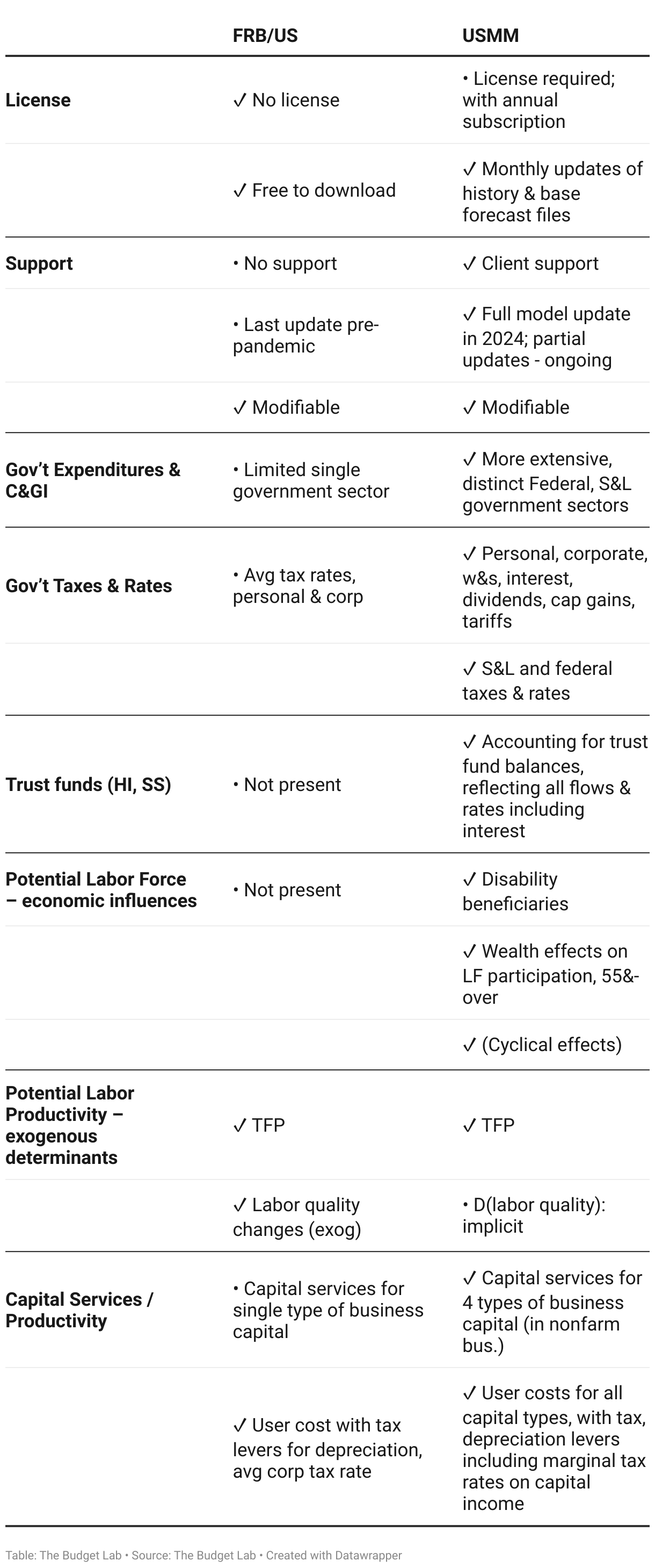
The balances of major government trust funds for social insurance are modeled in USMM, reflecting inflows and outflows, including interest. The trust funds are not present in FRB/US.
There are broad similarities but also important differences in the modeling of potential output between FRB/US and USMM. In both models, labor productivity reflects both exogenous contributions (from e.g., total factor productivity) and endogenous contributions from capital-deepening; in the case of USMM, capital-deepening reflects the weighted growth in each of the various business capital stocks, in contrast to the single “capital stock” in FRB/US. This is potentially important to reflect the differential growth in capital stocks that possess different marginal products of capital.
An important area of difference between the two models is in expectations that influence behavior in financial markets. In FRB/US, expectations can either be modeled as perfect foresight or determined with a small-scale vector autoregression. As noted above, in USMM monetary policy expectations are determined in a structural fashion to reflect investors’ perceptions of how the Federal Reserve will respond to departures from its goals for inflation and labor markets. In the section on implementation, we discuss how we adapted USMM to reflect the influence of expectations of long-term fiscal policy changes on interest rates.
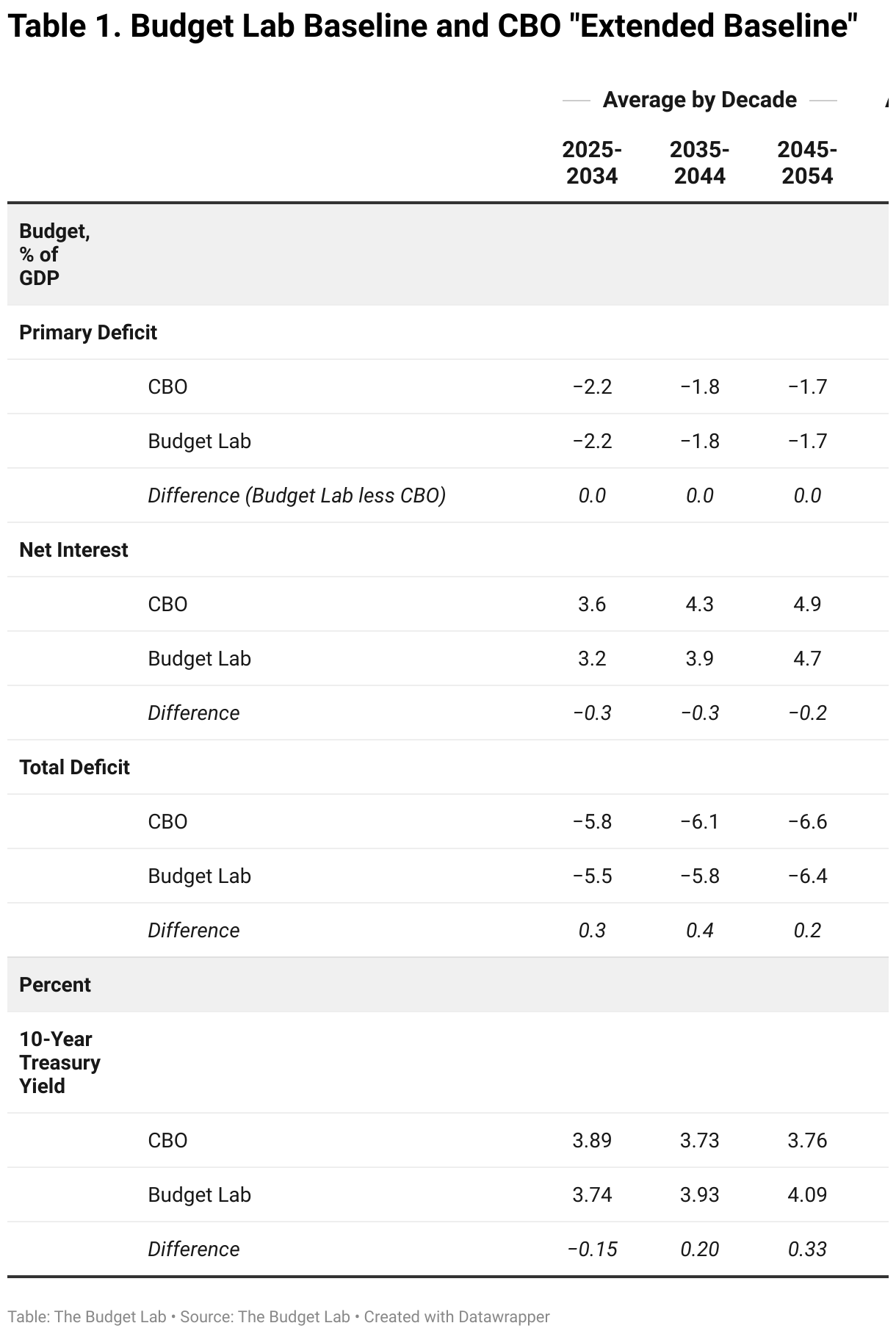
Baseline Aligned with CBO
For purposes of estimating the impact the OBBBA, we conducted our analysis relative to a 30-year baseline scenario constructed at The Budget Lab with USMM. Our baseline scenario is similar to CBO’s “extended baseline” in several important respects.
- Like CBO’s baseline, it is a “current law” projection.
- It is conditioned on the same population and demographic assumptions.
- It is based on the same estimate of the NAIRU.
- The size of the labor force is virtually identical to CBO’s projection.
- It reflects credible monetary policy that minimizes departures of inflation from the Fed’s 2% (PCE) inflation target and the unemployment rate from the NAIRU.
- Our baseline was constructed to generate paths for federal revenues and noninterest outlays that are similar to CBO’s extended baseline, so primary deficits are similar.
- As with CBO’s January 2025 baseline, our baseline does not include recently announced tariffs.
In USMM, the federal government is presented on the basis of the National Income and Product Accounts (NIPAs).3 It was necessary first to translate CBO’s extended baseline budget projections to a NIPA basis as a set of references for constructing the baseline in USMM. CBO periodically provides updated translations of its budget projections to be consistent with the NIPAs for the first decade of the forecast. We used relationships suggested by the most recently available 10-year CBO translation to convert budget projections beyond the first 10 years (that is, from 2035 to 2054) to a NIPA basis. In simulation with USMM, we adjusted effective tax rates and federal expenditures in USMM so that projections for revenues, non-interest outlays, and primary deficits were close to CBO’s 30-year extended baseline converted to a NIPA basis.4 When simulating a baseline in USMM, we aligned with both broad budget aggregates of CBO’s extended baseline, such as primary deficits, as well as key macroeconomic variables including the labor force, unemployment, and inflation.
After constructing the baseline scenario in USMM, NIPA budget figures were converted to a budget basis for direct comparison to CBO’s published extended baseline. The table nearby compares CBO’s extended baseline to our 30-year current-law baseline for deficits, net interest, and the key 10-year Treasury yield. Measured on a percent-of-nominal-GDP basis, our projections for primary deficits averaged by decade are equal to CBO’s. Our projection for net interest is slightly lower because we allow interest rates to ease more than CBO in the first few years. Around the time that TCJA expires in the baseline, in 2026, we allow the Fed to respond by lowering interest rates to minimize departures from full employment and to respond to disinflationary pressures. As noted previously, federal net interest outlays respond gradually to lower trajectories for market interest rates in the first few years of our baseline, because on average only approximately 30 to 40% of marketable federal debt matures in a given year. The lower trajectory for net interest in our baseline results in smaller total deficits than for CBO. However, the difference between the baseline deficit projections shrinks in the long run, as explained next.
Beyond the short run, we allow increases in the ratio of debt/GDP to be reflected in moderately higher interest rates as the Fed continues to target 2% inflation and unemployment at NAIRU. (Currently our modeling has interest rates more sensitive to an increase in debt/GDP than CBO’s appears to.) This results in a path for the 10-year yield that rises above CBO’s beginning in 2030 and continuing through the remainder of the projections. With a lag, the longer-run increase in interest rates in our baseline generates slightly faster growth of net interest than in CBO’s baseline, so the gaps in the levels of net interest narrow slowly.
Monetary Policy
When constructing the baseline simulation, we adapted the monetary policy block in USMM to ensure the successful pursuit of the Fed’s dual-mandate objectives to promote inflation and inflation expectations at 2% and maximum sustainable employment. This is consistent with CBO’s baseline.
In USMM, the federal funds rate is modeled with a Taylor-type policy rule with inertia, subject to the zero lower bound.5 Monetary policy expectations — market expectations of the federal funds rate over the horizon covered by longer-term Treasury instruments such as the 10-year Treasury note — are modeled to reflect market participants’ expectations that the Federal Reserve would adjust the federal funds rate in the future to respond to deviations of inflation and inflation expectations from its 2% longer-run objective and to differences between the unemployment rate and the NAIRU. (Expectations of future short-term interest rates influence longer-term interest rates such as the 10-year Treasury yield.)
In preliminary analysis with USMM, we observed that the model’s specification for monetary policy and monetary policy expectations caused interest rates to move in the anticipated directions — higher when inflation exceeded 2% or lower when the unemployment rate rose above the NAIRU, for example. However, the model did not always close the gaps to the policy benchmarks even after several years.
To construct our baseline, we felt it useful to manage the simulation so that inflation did converge to 2% and the unemployment rate tracked the NAIRU after short-run cyclical influences died out as these are the stated objectives of the Federal Reserve. To achieve this modeling objective, in simulation we adjusted the federal funds rate and monetary policy expectations to respond more vigorously than in the USMM equations to deviations from 2% inflation and a nonzero unemployment gap. Our procedure effectively strengthened the response of monetary policy to deviations from policy targets to be consistent with the assumptions of Fed credibility and efficacy. With this simulation strategy, we succeeded in eliminating long-run deviations of inflation from 2% and the unemployment rate from the NAIRU, similar to features in CBO’s projections.6 Our procedure ensured that over the longer run, the simulated trajectories for interest rates would be aligned with the model’s implicit path for the equilibrium real interest rate — “r-star” in common parlance.
Estimating the Dynamic Impacts of H.R. 1., the "One Big Beautiful Bill Act" (OBBBA)
Budget Impacts and Assumptions
We used USMM to estimate the full dynamic, macroeconomic effects of enacting the OBBBA. We used our conventional budget scores consistent with our tax simulator to estimate changes in effective and marginal federal tax rates in USMM, and parameters that affect cost recovery for business fixed investment such as R&D and equipment; and we used conventional scores of spending changes to develop equivalent adjustments to relevant components of federal spending in USMM. With these tax and spending inputs we simulated USMM for 30 years, then observed the difference between this simulation and the baseline described above to obtain an estimate of the full dynamic effects of enacting the OBBBA. These are the results discussed at length in our report. In this section we explain how we implemented the simulation to estimate dynamic impacts.
Focusing on the tax side, our tax simulator was employed to estimate changes to weighted average effective federal tax rates for personal income and corporate profits relative to their baseline settings that, when applied to USMM, resulted in the same mechanical impacts on federal revenues. For tax provisions that we cannot model using our simulator, we used the revenue estimates from the Joint Committee on Taxation. The tax simulator was also used to estimate changes in marginal tax rates on wages and salaries and on the several types of capital income tracked in USMM. Tax rates were estimated for each of 30 years. Our model for simulating cost recovery policy was used to generate paths for the average effective present value of depreciation allowances (PVDAs) for the several types of business capital in USMM: intellectual property products, computers, non-computer equipment, and nonresidential structures. We adjusted relevant levers in USMM, such as tax service lives, so that USMM-simulated PVDAs aligned with those determined by our tax simulator. The attention to these details allowed us to employ USMM to simulate the macroeconomic impacts on business fixed investment and capital accumulation of both temporary and permanent elements of the OBBBA that affect business cost recovery and the taxation of profits and capital income.7
On the expenditure side of the federal budget, we allocated the impacts of OBBBA’s spending provisions to their corresponding components of federal expenditures in the NIPAs on a year-by-year basis so that they could be reflected in the relevant components in USMM.8 By a wide margin, the largest cumulative impacts were reductions of federal grants-in-aid to state & local governments for health care. Reductions were also made to federal expenditures for the purchase of intermediate goods and services, and to federal transfers.9 10
Financial Considerations When Simulating the OBBBA
Enactment of the OBBBA would be associated with a substantially larger increase in federal debt to GDP than if it had not been enacted, engendering upward pressure on interest rates and substantially increasing debt service costs. Concerns about the political will to address debt sustainability and heightened risk of financial fragility could cause investors to increase risk pricing on a wide variety of US assets, including private ones such as stocks and corporate bonds. This could be reflected in larger risk premia on private debt instruments, such as corporate bonds, and increases in the equity risk premium.
To reflect these pressures, we made adjustments that resulted in wider risk spreads on private borrowing relative to yields on benchmark Treasuries — on corporate bonds and mortgages, for example; a gradual increase in the equity risk premium; and an increase in the term premium on the 10-year Treasury note. Each of these adjustments were implemented gradually relative to baseline settings and were moderate in historical context:11
- Through ad-factoring, the term premium on the 10-year Treasury yield was boosted gradually, with an impact that reached 25 basis points in 2054. (The overall impact on the term premium was affected by additional factors discussed below.)
- The equity risk premium was raised relative to its baseline path in a gradual fashion, reaching 0.4 percentage point in 2054. Increases in the equity risk premium, all else equal, are associated with lower dividend-price ratios on the S&P 500 and smaller capital gains on equity. They are also associated with a smaller term premium.12
- Risk spreads on Baa corporate bonds and the conventional mortgage rate relative to comparable Treasuries were boosted gradually through ad-factoring by amounts that reached 24 basis points and 20 basis points, respectively, in 2054.
In isolation, changes in parameters related to risk pricing are associated with a tightening of financial conditions. In equilibrium, their impacts on GDP, inflation, and federal outlays for net interest are generally offset by an implicit reduction in the equilibrium federal funds rate.
Strengthening Monetary Policy Responses
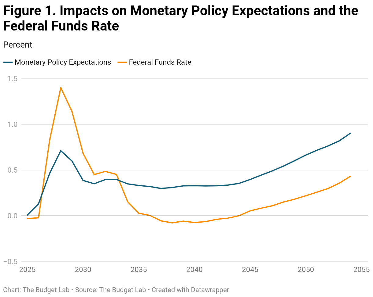
Similar to our treatment of monetary policy in the construction of the current-policy baseline described previously, for the alternative that reflects enactment of the OBBBA, we augmented the responses of the federal funds rate and monetary policy expectations to deviations from the Fed’s policy targets, resulting in a simulation where inflation remains close to 2% and the unemployment rate close to the NAIRU after short-run cyclical factors run their course in the first few years. The nearby chart depicts the resulting path for the differences in the federal funds rate and 10-year monetary policy expectations between the OBBBA simulation and baseline. Relative to baseline, monetary policy expectations are 90 basis points higher in 2054 and the federal funds rate is 43 basis points higher. The larger response of monetary policy expectations reflects investors’ expectations that additional rate increases will be needed beyond the horizon of the simulation to keep inflation anchored at 2%. These effects can be viewed as consistent with a fiscally-driven increase in r*.
Federal Interest Payments and Foreign Ownership of Government Debt
Changes in fiscal policy that result in lasting increases in primary deficits raise the interest costs associated with government debt, in equilibrium further raising deficits and debts, which further adds to the increase in interest costs. Interest payments flow to either domestic or foreign recipients, with potential implications for saving, spending, and interest rates. Model judgments that influence these channels can exert a significant impact on the dynamic budgetary and macroeconomic impacts of the original policy change.
When designing the simulation experiment to assess the impacts of enacting the OBBBA, we made several decisions that influenced feedback related to interest costs.
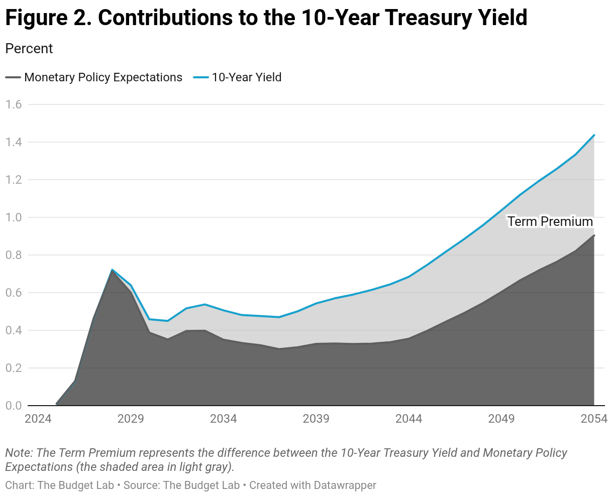
- We assumed a gradual increase in the average time remaining to maturity of federal debt, from 68 months in 2025 to 75 months in 2054. This was motivated by the observation that the average time remaining to maturity of the stock of debt tends to rise when debt is growing, unless offset by a reduction in the average maturity of newly issued debt. Lengthening the average remaining maturity of federal debt has two material impacts in USMM: (1) it slows the adjustment of the average effective interest rate on federal debt to changes in market interest rates; and (2) it makes a positive contribution to the term premium that rises slowly over time. The assumed increase in the average remaining time to maturity contributed 34 basis points to the 10-year term premium as of 2054. This is in addition to other factors influencing the term premium described previously. A chart nearby depicts the impacts from all sources on the 10-year term premium when simulating the OBBBA.
- We further slowed the adjustment of the average effective interest rate on federal debt to changes in market interest rates through ad-factoring to reflect a judgment that the effective interest rate might respond more slowly than suggested by USMM, perhaps reflecting shifts in issuance patterns by the Treasury. With these adjustments and relative to baseline, the average effective interest rate rose gradually throughout most of the 30-year simulation, reaching a difference of 78 basis points in 2054, approximately one-half as large as the increase in the 10-year Treasury yield (144 basis points) and larger than the increase in the federal funds rate at the same horizon (43 basis points in 2054). Had we not imposed some judgmental restraint on the average effective interest rate, net interest costs to the federal government would have been higher in simulation, potentially boosting consumer spending that would have forced up market interest rates in equilibrium by even more than in our estimate, thereby engendering greater crowding out.
- We held steady at its recent historical level (28%) the proportion of Treasury debt held by foreigners. Domestic investors hold the remaining portion of debt and thus receive a large share of the additional interest income implied by higher debt and interest rates.
Consumer Spending Out of Interest Income
Except to the extent that it is otherwise offset, the increase in interest payments received by domestic holders of federal debt would result in a substantial increase in consumer spending that boosts aggregate demand, raises real GDP and employment, and generates inflationary pressure that the Fed would be obliged to counteract through higher real interest rates.13 The increase in total net interest (versus baseline) we estimate with OBBBA rises over time, reaching 3.3% of GDP in 2054. In our modeling, the ratio of interest payments received by domestic holders to GDP would rise to 6.5% in 2054, 2.4 percentage points higher than in the baseline scenario.
We assume that the personal saving rate would increase as debt rises persistently relative to incomes, moderating some of the spending impact from increases in interest income of households. To achieve this result, we offset a portion of the spending impact of the interest-income channel through negative ad-factoring of consumer spending. With this adjustment, the personal saving rate rises relative to baseline, reaching a difference of 3.0 percentage points in 2054.14
Our management of levers related to the effective interest rate on federal debt, the ownership of federal debt, and the feedback onto spending, saving, and GDP differs from our 2024 analysis of extending the Tax Cuts and Jobs Act. For the prior analysis, we assumed that the entire increase in federal interest payments went to the rest-of-world, implying no increase in interest income of US residents. This assumption shut down feedback from debt to interest income that would boost domestic consumption (unless completely offset by more domestic saving) and that in equilibrium puts upward pressure on US interest rates. This is a key issue when conducting long-run fiscal experiments designed to estimate the impacts of major legislation such as the budget bill. Assuming that all of the increase in net interest flows to the rest of the world eliminates an important channel for affecting the equilibrium real interest rate (r-star). Had we managed the simulation of the OBBBA in the same fashion as we employed in 2024, increases in interest rates would have been much smaller to reflect less income that would support aggregate demand and generate inflationary pressures. Increases in deficits and debts would have been smaller as well than those that we currently show.
Conclusion and Future Steps
Implementing a fully articulated, 30-year simulation with a large macroeconomic forecasting model such as FRB/US or USMM is a challenging task, especially when estimating the impacts of a substantial fiscal policy change on the scale of the OBBBA. The simulation results reflect importantly both the mathematical structure of the model and the many judgments made in implementation. We view all of those judgments and our modeling choices as subject to change. We expect to continue to refine and improve our methodology in response to experience and to feedback, which we welcome. The Budget Lab feels that assumptions around how interest rates respond to increased debt and deficits are important areas of future research and refinement.
Footnotes
- The short-run slope of the Phillips Curve, in USMM, is shallow, with a coefficient on the unemployment gap of 0.06.
- Below we describe how we adapted the model to generate paths for expected short-term interest rates consistent with long-term fiscal policy changes.
- More information on the presentation of the federal government sector in the NIPAs is available in Baker, B., and P. Kelly, “A Primer on BEA’s Government Accounts,” Bureau of Economic Analysis, March 2008.
- We aligned approximately on the breakdown between taxes on corporate profits and on personal income in CBO’s projections while more closely matching total revenues projections.
- The equation that determines the federal funds rate in USMM displays a much lower degree of inertia (0.3) than in some alternative versions, such as the inertial version of the policy rule maintained by the Federal Reserve Bank of Cleveland (0.8).
- We used a similar procedure for implementing monetary policy assumptions when constructing the alternative scenario in the next section.
- We estimated, with USMM, that nonresidential fixed investment would rise modestly above baseline in response to more favorable cost recovery provisions in the OBBBA. Eventually, however, the effects of those provisions were more than offset by crowding out associated with higher real interest rates. In 2054, the level of real nonresidential fixed investment was 14% lower than in the baseline projection. Real business capital stocks in 2054 were from 4% to 11% below their baseline values.
- USMM contains approximately two dozen distinct components of federal expenditures.
- We reduced S&L expenditures for health care to match the reduction in Federal grants-in-aid to avoid unsustainable changes to the aggregate budget balance of the state and local sector.
- We judged that most of the Education Committee’s budget impact in OBBBA is related to student loans, which we allocated to Federal transfers to persons. The largest impact of this provision was in the first year (2025), during which we lowered our assumption for federal transfers to persons by some $160 billion at an annual rate, relative to the baseline. In USMM, the marginal propensity to consume out of transfer income is equal to one, so reductions in government transfers to persons contributed to a reduction in personal consumption expenditures and a modest, temporary reduction of GDP in the first year before they were outweighed by the stimulative effects of tax cuts that ramp up over several quarters. In terms of fiscal-year averages, GDP is 0.1% lower than baseline in 2025, equal to baseline (0.0%) in 2026, and above baseline from 2027 to 2032 with a peak increase of 0.7% in 2027.
- A similar situation — with debt/GDP projected to far exceed 150% of GDP within a few decades — is unprecedented in modern US history, implying there is no clear historical episode to help calibrate the size of these changes. We feel this supports our decision to generate only moderately higher values for risk premia than in the baseline. We acknowledge that there is a large degree of uncertainty about how large such effects might be.
- In USMM, the equity risk premium influences longer-term interest rates through the difference between its current level and its trailing 12-quarter average. Positive values for this difference are associated with a negative impact on term premia, reflecting flight-to-safety considerations, and positive impacts on risk spreads for corporate bonds and residential mortgages. The increment to the equity risk premium we applied when simulating the OBBBA was entered in a gradual fashion, so secondary impacts were small relative to the direct effects described in the main text. They did not alter the conclusion that the adjustments described in this section contributed to tighter financial conditions that, at the margin, put downward pressure on the equilibrium real federal funds rate that was more than offset by upward pressure from protracted fiscal stimulus.
- In USMM, the marginal propensity to consume out of asset income, including interest income, is set at 0.44.
- Similar results can be obtained by lowering the marginal propensity to consume out of asset income.